Advanced Octrees 4: finding neighbor nodes

Introduction

Welcome to part four of the the Advanced Octrees series. Here you can find part one, two and three. In this part I show you how to access neighbor nodes in Quadtrees. The algorithm can be naturally extended to Octrees, but it’s easier to understand and code in just two dimensions. Neighbors are such nodes that either share an edge in horizontal (west, east) or vertical (north, south) direction, or that share a vertex in one of the four diagonal directions (north-west, north-east, south-west, south-east). See the figure below for an illustration. The node of which we want to find the neighbors is colored green. In the following this node is called source node. The neighbor nodes are colored red and labeled with the corresponding direction.

In the literature Quadtree neighbor finding algorithms are distinguished by two properties:

1. Does the algorithm operate on pointer-based Quadtrees or on linear Quadtrees? Read up on different Quadtree representations in part two of this series. The algorithm discussed in this post is based on a pointer representation.
2. Can the algorithm only find neighbors of equal or greater size, or can it also find neighbors of smaller size. We’ll see later that finding neighbors of smaller size is somewhat harder. Greater / equal / smaller refers to the difference in tree level between the source node and the neighbor nodes.

The figure below shows examples of neighbor relationships in north direction between nodes on different tree levels. Note, that a node can have more than one neighbor per direction if the sub-tree on the other side of the north edge is deeper than the sub-tree of the source node.

Algorithm

The input to the algorithm is a direction and an arbitrary Quadtree node (inner of leaf). The output is a list of neighbor nodes in the given direction. The neighbors can be of greater size, equal size or smaller size (see previous figure). The algorithm is symmetric with respect to the direction. That’s why I only show an implementation for the north direction. It should be easy to extend the implementation to the other seven directions.

The neighbor finding happens in two steps. In step 1 we search for a neighbor node of greater or equal size (yellow). If such a node can be found we perform the second step, in which we traverse the sub-tree of the neighbor node found in step 1 to find all neighbors of smaller size. The two steps are illustrated in the figure below.

So how to find the neighbor of greater or equal size? Starting from the source node the algorithm traverses up the tree as long as the current node is not a south child of the parent, or the root is reached. After that the algorithm unrolls the recursion descending downwards always picking the south node. The node the recursion stops at is the north neighbor of the source node. This node is always on the same tree level as the source node, or further up the tree. Because the source node can be in the west or in the east, there’s a case distinction necessary to handle both possibilities.

Below is an implementation in Python. The code uses a pointer based Quadtree data structure, in which every node consists of a parent and four children. The children array is indexed using the constants NW, NE, SW and SE. The full code can be found on Github.

def get_neighbor_of_greater_or_equal_size(self, direction):   
  if direction == self.Direction.N:       
    if self.parent is None: # Reached root?
      return None
    if self.parent.children[self.Child.SW] == self: # Is 'self' SW child?
      return self.parent.children[self.Child.NW]
    if self.parent.children[self.Child.SE] == self: # Is 'self' SE child?
      return self.parent.children[self.Child.NE]

    node = self.parent.get_neighbor_of_greater_or_same_size(direction)
    if node is None or node.is_leaf():
      return node

    # 'self' is guaranteed to be a north child
    return (node.children[self.Child.SW]
            if self.parent.children[self.Child.NW] == self # Is 'self' NW child?
            else node.children[self.Child.SE])
  else:
    # TODO: implement symmetric to NORTH case

In step 2 we use the neighbor node obtained in step 1 to find neighbors of smaller size by recursively descending the tree in south direction until we reach the leaf nodes. On the way we always keep both, the south west and the south east node, because any node lower in the tree than the neighbor node from step 2 is smaller than the source node and therefore a neighbor candidate.

def find_neighbors_of_smaller_size(self, neighbor, direction):   
  candidates = [] if neighbor is None else [neighbor]
  neighbors = []

  if direction == self.Direction.N:
    while len(candidates) > 0:
      if candidates[0].is_leaf():
        neighbors.append(candidates[0])
      else:
        candidates.append(candidates[0].children[self.Child.SW])
        candidates.append(candidates[0].children[self.Child.SE])

      candidates.remove(candidates[0])

    return neighbors
  else:
    # TODO: implement other directions symmetric to NORTH case

Finally, we combine the functions from step 1 and 2 to get the complete neighbor finding function.

def get_neighbors(self, direction):   
  neighbor = self.get_neighbor_of_greater_or_equal_size(direction)
  neighbors = self.find_neighbors_of_smaller_size(neighbor, direction)
  return neighbors

Complexity

The complexity of this algorithm is bounded by the depth of the Quadtree. In the worst-case the source node and its neighbors are on the last tree level but their first common ancestor is only the root node. This is the case for any node that lies directly below/above or left/right of the line splitting the root node horizontally/vertically. See the following picture for an illustration.

Test-and-set spinlocks

In my previous blog post I wrote about the most important properties of spinlocks and why they matter. This time I’ll present the first out of three concrete spinlock implementations in C++11 for x86 processors. I’m assuming that you’ve read the first post. You can find all source code in this Github repository.

Introduction

The Test-And-Set (TAS) Lock is the simplest possible spinlock implementation. It uses a single shared memory location for synchronization, which indicates if the lock is taken or not. The memory location is updated using a test-and-set (TAS) operation. TAS atomically writes to the memory location and returns its old value in a single indivisible step. Actually, the name test-and-set is a little misleading, because the caller is responsible for testing if the operation has succeeded or not. The TAS Lock is not fair as it doesn’t guarantee FIFO ordering amongst the threads competing for the lock.

In C++11 std::atomic_bool::exchange() can be used to perform a TAS operation on an std::atomic_bool synchronization variable. On x86 CPUs std::atomic::exchange() is turned into the LOCK XCHG instruction (side note: the LOCK prefix is implicit and not strictly required, because there’s no non-atomic version of XCHG). The following code implements the described TAS Lock.

class TasSpinLock
{
public:
    ALWAYS_INLINE void Enter()
    {
        // atomic_bool::exchange() returns previous value of Locked
        while (Locked.exchange(true, std::memory_order_acquire) == true);
    }

    ALWAYS_INLINE void Leave()
    {
        Locked.store(false, std::memory_order_release);
    }

private:
    alignas(CACHELINE_SIZE) std::atomic_bool Locked = {false};
};

static_assert(sizeof(TasSpinLock) == CACHELINE_SIZE, "");

The TasSpinLock::Locked flag is cache line size padded using alignas to prevent false sharing. You can remove the padding, e.g. in memory-limited environments, when false sharing is not an issue.

The test-and-test-and-set optimization

While the TAS Lock is extremely easy to implement, its scalability is very bad. Already with just a few threads competing for the lock, the amount of required cache line invalidations to acquire/release the lock quickly degrades performance. The problem is two-fold.

1. std::atomic_bool::exchange() always invalidates the cache line Locked resides in, regardless of whether it succeeded in updating Locked or not.
2. When the spinlock is released, all waiting threads simultaneously try to acquire it. This is sometimes referred to as Thundering Herd problem. Acquiring the lock means first invalidating the cache line copy of all threads waiting for the lock and then reading the valid cache line copy from the core which released the lock. With t threads this results in O(t) memory bus transactions.

The latter issue is inherent to TAS Locks, because just a single synchronization variable is used and shared between all threads. However, the first issue can be fixed by testing if the lock is free before calling exchange(). First testing if the lock is free only loads the synchronization variable and therefore doesn’t cause a cache line invalidation. This spinlock variant is called Test-And-Test-And-Set (TTAS) Lock. The improved Enter() method looks like this:

ALWAYS_INLINE void TTasSpinLock::Enter()
{
    do
        WaitUntilLockIsFree();
    while (Locked.exchange(true, std::memory_order_acquire) == true);
}

ALWAYS_INLINE void TTasSpinLock::WaitUntilLockIsFree() const
{
    while (Locked.load(std::memory_order_relaxed) == true);
}

Exponential back-off

The TTAS Lock successfully reduces the amount of cache line invalidations occurring while the lock is trying to be acquired. However, as soon as the lock is released, again all threads try to update the Locked flag. If a thread sees that the lock is free, but fails acquiring it subsequently because some other thread was faster, the lock is most probably under high contention. In this situation it can help to wait for a short time to let other threads finish before trying to enter the critical section (CS) again.

Waiting a short time without trying to acquire the lock reduces the number of threads simultaneously competing for the lock. The larger the number of unsuccessful retries, the higher the lock contention and the longer the thread should back-off. Experiments have shown that a good strategy is to back-off exponentially; similar to the congestion avoidance mechanism used in the Ethernet protocol. To avoid threads running in lock step the initial wait time is randomized.

ALWAYS_INLINE static void BackoffExp(size_t &curMaxIters)
{
    assert(curMaxIters > 0);

    thread_local std::uniform_int_distribution<size_t> dist;
    thread_local std::minstd_rand gen(std::random_device{}());
    const size_t spinIters = dist(gen, decltype(dist)::param_type{0, curMaxIters});

    curMaxIters = std::min(2*curMaxIters, MAX_BACKOFF_ITERS);
    for (volatile size_t i=0; i<spinIters; i++); // Avoid being optimized out!
}

ALWAYS_INLINE void ExpBoTTasSpinLock::Enter()
{
    size_t curMaxIters = MIN_BACKOFF_ITERS;

    while (true)
    {
        // Not strictly required but doesn't hurt
        WaitUntilLockIsFree();

        if (Locked.exchange(true, std::memory_order_acquire) == true)
            BackoffExp(curMaxIters); // Couldn't acquire lock => back-off
        else
            break; // Acquired lock => done
    }
}

The downside of waiting is that it renders the lock even unfairer than it is already. Threads that have been attempting to acquire the lock longest are also backing-off longest. Consequently, newly arriving threads have a higher chance to acquire the lock than older threads. On top of that threads might back-off for too long, causing the CS to be underutilized. Furthermore, there are unfortunately no single best values for MIN_BACKOFF_ITERS and MAX_BACKOFF_ITERS. Optimally, they’re determined experimentally depending on the workload (contention, size of CS).

Pausing and sleeping

There are two more improvements we can do. First, according to the Intel Architectures Optimization Reference Manual, adding a PAUSE instruction to the body of all spin loops improves performance on Pentium 4 CPUs and later. The PAUSE instruction provides a hint to the CPU that the code being executed is a spin-wait loop. PAUSE is backwards compatible and turns into a NOP instruction on older CPUs. There are three reasons why using PAUSE improves performance:

• It avoids memory order violations which result in expensive pipeline flushes, because the CPU doesn’t go ahead to fill its pipeline with speculatively executed load and compare instructions.
• It gives the other hardware thread time to execute on simultaneous multi-threading (SMT) processors (e.g. Intel’s Hyper Threading).
• It adds a slight delay to the spin loop, which synchronizes it with the system’s memory bus frequency. This frequency is typically much lower than the frequency of the CPU, which in turn reduces power consumption considerably.

The second improvement is to stop spinning, put the thread to sleep and reschedule if the the lock doesn’t become available after some time. The important bit here is to not yield (sched_yield() on Linux, SwitchToThread() on Windows, or more generally std::this_thread::yield() in C++11), but to explicitly put the thread to sleep for a short period of time. This ensures that the thread is really paused for some time and isn’t immediately run again by the scheduler if there’s no other thread available in the scheduler’s run queue. This is especially important on SMT processors where every two logical cores share most of the execution units. Only when the thread is really sleeping the other logical core can fully make use of the shared execution units. The following TTAS Lock implementation uses the PAUSE instruction and sleeps for 500us if the lock isn’t released within MAX_WAIT_ITERS iterations. There’s no single best value for MAX_WAIT_ITERS. Ideally, it’s chosen experimentally like the MIN_BACKOFF_ITERS and MAX_BACKOFF_ITERS constants from before.

ALWAYS_INLINE static void CpuRelax()
{
#if (COMPILER == MVCC)
    _mm_pause();
#elif (COMPILER == GCC || COMPILER == LLVM)
    asm("pause");
#endif
}

ALWAYS_INLINE static void YieldSleep()
{
    // Don't yield but sleep to ensure that the thread is not
    // immediately run again in case scheduler's run queue is empty
    using namespace std::chrono;
    std::this_thread::sleep_for(500us);
}

ALWAYS_INLINE static void BackoffExp(size_t &curMaxIters)
{
    ... Unchanged code not repeated, look above ...

    for (size_t i=0; i<spinIters; i++)
        CpuRelax();
}

ALWAYS_INLINE void ExpBoRelaxTTasSpinLock::WaitUntilLockIsFree() const
{
    size_t numIters = 0;

    while (Locked.load(std::memory_order_relaxed))
    {
        if (numIters < MAX_WAIT_ITERS)
        {
            CpuRelax();
            numIters++;
        }
        else
            YieldSleep();
    }
}

Performance comparison

The benchmark used to compare the different TAS Lock variants is extremely simple and should be taken with a grain of salt. It launches t threads, each competing for the lock and incrementing a global atomic counter inside the CS. This causes high lock contention, because all threads are trying to enter the lock at the same time. Though, it’s important to keep in mind that due to the lock’s lack of fairness, it’s entirely possible that the same thread acquires the lock multiple times in a row. I ran the benchmark on a dual socket NUMA system with two Intel Xeon E5-2630 v2 CPUs with 2.60 GHz. The CPUs support Hyper Threading which gives a total of 12 physical and 24 logical cores. The benchmark results are shown below.

The most interesting finding is that the amount of lock reacquisitions is a lot higher than I anticipated. This can be derived from the fact that all TTAS-based locks scale almost linearly, where typically the observed drop in performance for TAS-based locks is exponential. Large numbers of lock reacquisitions by the same thread reduces the amount of cache line invalidations and increases throughput. At the same time the latency of all other threads goes up, because they’re granted the lock later.

The TasSpinLock scales so much worse, even though lock reacquisiton happens, because while spinning the TAS operation causes cache line invalidations also if it doesn’t succeed in acquiring the lock. By looking at the difference between the TasSpinLock and the other TTAS-based versions, it’s highly visible how big the influence of cache line invalidations is on the lock’s performance.

Wrapup

The exponential back-off TTAS Lock tends to perform fairly well as long as the number of competing threads is low or lock reacquisitions boost throughput while increasing latency. It’s especially useful when it’s not known a priori that the number of competing threads is bounded by the number of cores in the system (in that case better scaling spinlock variants perform really badly as we’ll see in the next post). Beyond that, without padding the TTAS Lock just needs a single byte. The compact representation is useful in extremely memory-constrained environments or applications that require vast amounts of spinlocks; e.g. for fine-grained locking of lots of small pieces of data.

Important properties of spinlocks

Typically, when a thread tries to acquire an already locked mutex it will go to sleep and give up its time slice, allowing another thread to run immediately instead. If the duration for which the mutex is held is extremely short, the time for putting the waiting thread to sleep and waking it up again to retry can easily be longer. In such cases spinlocks can be used to increase performance, by continuously trying to acquire the lock without sleeping. Side note: Obviously, it makes no sense to use spinlocks in systems with a single CPU core. Polling for the spinlock to become available would only prevent the single available CPU core from running the other thread to release the lock.

To deep dive into the multitude of spinlock implementations, it’s crucial to understand what their key characteristics are. Generally, spinlocks can be grouped into fair and unfair as well as scalable and unscalable implementations. In addition, we look at the spinlock’s memory footprint. The three properties are discussed in more detail in the rest of this post.

For all the nitty-gritty architectural details of concrete C++11 spinlock implementations read the upcoming blog posts about Test-And-Set (TAS) Locks, Ticket Locks and MCS Locks. I’ll upload the source code to this Github repository.

Scalability

Existing spinlock variants have very different performance characteristics under contention. A lock is said to be contented when there are multiple threads concurrently trying to acquire the lock while it’s taken. The performance of unscalable spinlock implementations degrades as the number of threads trying to acquire the lock concurrently goes up. The performance of simple Ticket or TAS Locks for example drops exponentially with increasing numbers of threads. In contrast, scalable spinlock implementations – like e.g. the MCS Lock – exhibit no degradation in performance even for large numbers of threads. The scalability graph of the optimal spinlock vs the Ticket Lock is depicted in the graph below.

Crucial for the scalability of spinlocks is the amount of cache line invalidations which take place when the lock is acquired and released. Cache line invalidations take place when e.g. a thread modifies a synchronization variable while leaving a critical section (CS) on which other threads are polling at the same time. Suddenly, cache line copies stored in caches of other CPU cores are not valid anymore. Accordingly, these cache lines must be invalidated and reobtained from the CPU core’s cache which modified it. Thus, the number of cache line invalidations which occur when the spinlock is acquired/released is often used as a metric to compare spinlock implementations with each other. Usually, scalable spinlocks require O(1) many cache line invalidations to acquire/release the lock, while unscalable spinlocks require O(#threads) many.

Advanced scalable spinlock implementations may not only take the total number of CPU cores in a system into account, but also the details of the underlying cache coherency mechanism. For example in systems with multiple CPUs and non-uniform memory access times (NUMA), inter-core communication costs may vary greatly. For example in a NUMA system with multiple multi-core CPUs it’s entirely possible to pass a lock to another core within in the same CPU in less time than to a core of another CPU.

Fairness

Fair spinlocks guarantee that the same thread may never reacquire the lock if there are other threads trying to acquire the same lock at the same time. Fair spinlocks maintain a first-in-first-out (FIFO) order among the threads attempting to acquire the lock.

Often, unfair spinlocks trade latency for throughput, while fair spinlocks trade throughput for latency. Consider the following example. Let’s say we’re running t threads each performing n/t loop iterations in which they try to enter a CS. When using an unfair spinlock, in the worst case (at least in theory) every thread could enter the CS n/t times in a row instead of alternating with lock acquisition between threads. In certain scenarios this can boost throughput considerably, because the number of expensive cache line invalidations is reduced. However, the time until any other thread may enter the CS rises. In theory this can lead to starvation. In practice the cache coherency protocol should ensure that no starvation occurs.

Typically, the performance of fair spinlocks drops extremely when the number of threads competing for the same lock is greater than the number of CPU cores in the system. The reason for this is that the thread which is next in the sequence to acquire the lock might be sleeping. In contrast to unfair spinlocks, during the time the next thread is sleeping no other thread can acquire the lock because of the strict acquisition order guaranteed by the fair lock. This property is sometimes referred to as preemption intolerance.

Memory footprint

Generally, the required memory to store l spinlocks can depend on the number of threads t which are using the lock. While some spinlock implementations require only constant memory for t threads, other’s memory footprint scales linearly with the number of threads. The amount of needed memory to store a spinlock mostly doesn’t matter, because the memory footprint for the majority of locks is in the order of a few dozen bytes per thread. Mostly it’s a multiple of the CPU’s cache line size to account for false sharing. However, there are cases where the memory footprint plays an important role. Examples are extremely memory-constrained environments or applications that require vast amounts of spinlocks e.g. for fine-grained locking of lots of small pieces of data.

Splitting an arbitrary polygon by a line

In this post I present an algorithm for splitting an arbitrary, simple polygon by a line. My implementation is based on ideas from the article Spatial Partitioning of a Polygon by a Plane by George Vanecek, published in the book Graphics Gems V. The intention behind this post is covering all the details which the original article omitted. All polygons are assumed to be oriented counter clockwise. You can find the full source code of my implementation in this github repository.

Introduction

Splitting a polygon by a line is very closely related to clipping a polygon against a clip region, like a rectangle or another polygon. Splitting a polygon is easier and at the same time harder than clipping a polygon. It’s easier because you only clip against a single line and it’s harder because the resulting polygons cannot simply be discarded. It turns out, that splitting convex polygons is a lot easier than splitting concave polygons. The reason is that splitting convex polygons results in at most two new polygons, whereas splitting concave polygons can result in arbitrary many new polygons. Look at the following figure for an illustration.

Coming up with a correct implementation for concave polygons is tricky, because there are many corner cases that must be considered. In the following, first, an algorithm for splitting convex polygons is outlined. Afterwards, the algorithm is extended to concave polygons.

Convex polygons

Splitting convex polygons is pretty simple. Essentially, one iterates over the polygon’s vertices, checks on which side of the split line they lie and adds them accordingly either to the left or the right result polygon. When an edge crosses the split line, additionally, the intersection point must be added to both result polygons. Special care must be taken when multiple successive vertices lie on the split line. In that case, due to the convexity property, the entire polygon lies either on the left-hand or on the right-hand side of the polygon. When for the second time a polygon edge crosses the split line, we know that the first half of the polygon is already completely split off.

Concave polygons

In contrast to splitting convex polygons it requires some more algorithmic effort to split concave polygons. When the split line crosses a concave polygon for the second time, it doesn’t necessarily mean that the first half of the polygon is now completely split off. On the contrary, it might be that another new polygon to be split off just opened. To account for that, first, I tried to iterate over the polygon edges while carrying along a stack of open polygons. Whenever, I came across a vertex which belonged to the open polygon on the top of the stack I knew it just closed. This approach worked out well until I tried accounting for all the corner cases. Finally, I decided to use the method from the article mentioned in the introduction.

Idea of the algorithm

The intersection points between the split line and the polygon are key to the splitting algorithm. By pairing up 2-tuples of intersection points along the split line, the edges closing the result polygons can be determined. Conceptually, every two intersection points along the split line form a pair of edges, each closing one side of two neighboring result polygons. In a perfect world, the intersection points could be easily paired up after sorting them along the split line, relative to the split line’s starting point (cf. the left figure below). Unfortunately, in the real world special care must be taken when the split line doesn’t cross a polygon edge in middle, but only touches the start and/or end vertex. In such cases the pairing up of source points (red) and destination points (green) along the split line gets trickier (cf. the figure in the middle blow). As you can see, only certain intersection points qualify as sources and destinations and some intersection points even qualify as both (yellow, cf. the right figure below). Luckily, it’s possible to account for all of these cases as we’ll see later.

Computing the intersection points

To ease the splitting process it’s helpful to represent the polygon as a doubly linked list. We compute the intersection points between the split line and the polygon by iterating over each polygon edge e and determining on which side of the split line the edge’s start vertex e.Start and end vertex e.End lies. If e.Start lies on the split line e is added to the array EdgesOnLine, which contains all edges starting on the split line. If e.Start and e.End lie on opposite sides of the split line, a new edge starting at the intersection point is inserted into the polygon and added to EdgesOnLine. The edges in this array are of interest, because they start at the intersection points with the split line. The algorithm is outlined below.

for (auto &e : poly)
{
    const LineSide sideStart = GetLineSide(SplitLine, e.Start);
    const LineSide sideEnd = GetLineSide(SplitLine, e.End);

    if (sideStart == LineSide::On)
    {
        EdgesOnLine.push_back(e);
    }
    else if (sideStart != sideEnd && sideEnd != LineSide::On)
    {
        Point2 ip = IntersectLines(SplitLine, e);
        Edge *newEdge = poly.InsertEdge(e, ip);
        EdgesOnLine.push_back(newEdge);
    }
}

Sorting the intersection points

After all polygon edges have been intersected with the split line, the edges in the EdgesOnLine array are sorted along the split line by the distance between their starting points and the starting point of the split line. Sorting the EdgesOnLine array is crucial for pairing up the source and the destination edges by simply iterating over the array as we see in the following section.

std::sort(EdgesOnLine.begin(), EdgesOnLine.end(), [&](PolyEdge *e0, PolyEdge *e1)
{
    return (CalcSignedDistance(line, e0->StartPos) <
            CalcSignedDistance(line, e1->StartPos));
});

As Glenn Burkhardt pointed out in a comment, the Euclidean distance cannot be used as distance metric because it’s unsigned. The Euclidean distance can only be used as long as the split line’s starting point lies outside the polygon. In that case all points are on the same side of the split line’s starting point and the Euclidean distance provides a strict order along the split line. However, if the split line’s starting point is inside the polygon, points on two different sides of the split line’s starting point will both have positive distances, which can result in wrong sort orders. A formula for computing the signed Euclidean distance between two points can be derived from the formula for scalar projections. In case of co-linear lines (angle between the two vectors is |1|) the result equals the signed distance along the split line.

static double CalcSignedDistance(const QLineF &line, const QPointF &p)
{
    return (p.x()-line.p1().x())*(line.p2().x()-line.p1().x())+
           (p.y()-line.p1().y())*(line.p2().y()-line.p1().y());
}

Pairing up edges

As we’ve seen before, all edges in the EdgesOnLine array are either source edges, destination edges or both. The edges must be classified accordingly, in order to be able to determine between which pairs of edges a bridge must be created to split the polygon. The source/destination classification is the most important part of the algorithm and the hardest to get right due to plenty of corner cases.

The starting point e.Start of any edge e in the EdgesOnLine array lies on the split line. Each edge e has a predecessor edge e.Prev and a successor edge e.Next. They can lie either on the left-hand side (L), on the right-hand side (R) or on the split line (O). Hence, there’s a total of nine configuration possibilities that must be evaluated in order to find out if an edge is a source, a destination or both. All nine configurations are depicted in the figure below. The vertex order is shown in the caption of each configuration.

I simply examined examples to classify each configuration as source, destination or both. The configurations’ winding orders are key for the classification. Imagine to move along the split line from its starting point to its endpoint. The winding order at the current intersection point indicates if we’re currently inside the polygon or not. Let’s take exemplary the LOR and ROL cases. The LOR case is only encountered when transitioning from the outside to the inside of a polygon. Hence, it’s a source configuration. In contrast, the ROL case is only encountered when transitioning from the inside of the polygon to the outside. Hence, it’s a destination configuration. Below are sample polygons depicted for the classification of each source and each destination configuration.

It follows that LOR, ROR, LOL, OOR and LOO are source configurations and ROL, ROR, LOL, ROO and OOL are destination configurations. Note, that these two sets are not disjoint: ROR and LOL are source and destination configurations. However, these two configurations can only be sources if they have served as destinations before!
Another corner case occurs when two successive edge starting points lie on the split line. Look at the example depicted in the figure below. There are two source edges (red) of which the second one must be used as source, even though it comes second in the EdgesOnLine array.

The EdgesOnLine array contains three edges: two source edges (red) and one destination edge (green). When splitting the polygon it’s crucial to pair up the the second and the third edge, not the first and the third. So how do we figure out which source edge to select when iterating over the EdgesOnLine array? It turns out that the distance between the starting points of the two successive source edges in question and the starting point of the split line can be used. An OOR and LOO source edge is only selected if the following candidate edge isn’t further away from the start of the split line and therefore closer to the next destination.

Rewiring the polygon

After we’ve figured out how the classification of source and destination edges works, we can finally formulate the algorithm to split concave polygons. All we need to do is to iterate over the EdgesOnLine array while pairing up source and destination edges. Each pair denotes one side of the polygon that has to be be split off. At this point it pays off that we use a linked list representation for the polygon. The current polygon side is split off by inserting two new edges between the source and the destination edge. Therefore, we iterate over the EdgesOnLine array, obtain the next source and the next destination edge and insert two new, oppositely oriented edges between them. This bridging operation is depicted in the following figure.

The main loop of the rewiring process is depicted below. For reasons of brevity only the overall structure is shown. For more details look into the full implementation in the github repository.

for (size_t i=0; i<EdgesOnLine.size(); i++)
{
    // find source edge
    PolyEdge *srcEdge = useSrc;

    for (; !srcEdge && i<EdgesOnLine.size(); i++)
    {
        // test conditions if current edge is a source
    }

    // find destination edge
    PolyEdge *dstEdge = nullptr;

    for (; !dstEdge && i<EdgesOnLine.size(); )
    {
        // test conditions if current edge is a destination
    }

    // bridge source and destination edges
    if (srcEdge && dstEdge)
        CreateBridge(srcEdge, dstEdge);
}

Collecting the result polygons

The final step, after all bridge edges have been inserted, is collecting the resulting polygons. For that purpose I use the Visited attribute in the edge data structure to indicate if an edge has been visited already and therefore, has been assigned already to one of the result polygons.

Advanced Octrees 3: non-static Octrees

Welcome to the third part of the Advanced Octrees series. Make sure you’ve also read part one and two. Typically, Octrees are constructed once for geometry which is known a priori and doesn’t change anymore (e.g. the level in a computer game). However, there are applications where objects are moving through the world, or objects located outside the Octree’s root cell must be inserted after the Octree has been constructed already. One approach would be to simply reconstruct the entire Octree from scratch each time it’s modified. While working, obviously, this turns very inefficient as soon as the Octree contains more than just a handful objects. In this post I present a way to relocate moving objects in already constructed Octrees, as well as a way to expand/shrink Octrees.

Relocate moving objects

An Octree which contains moving objects must be updated whenever a moving object starts straddling its parent cell’s bounding box. Usually, the number of moving objects is considerably smaller than the number of static objects. Thus, it can be advantageous to maintain two Octrees: one containing all static and one containing all moving objects. Instead of reconstructing the Octree from scratch, it’s much faster to relocate only the objects that have moved out of their parent cell.

Duplicating objects straddling cell boundaries works great for static scenes. However, in dynamic scenes keeping track of multiple references to the same object contained in multiple different nodes adds unnecessary complexity. Therefore, it’s better to place objects in the lowest Octree cell which completely encloses the object (see part one). That way a minimum amount of pointer information must be updated when a moving object transitions from one cell into another.

To update an Octree with moving objects, first, a list of all objects that have moved out of their parent cell is obtained. Each object in this list is pushed up the Octree until it ends up in a node which completely encloses it. The object must remain in this node, as long as it straddles any child cell’s bounding box of its new parent. However, when the object keeps on moving into the same direction, there will be the moment it’s again completely enclosed by one of its parent’s child cells. Therefore, finally, all previously pushed up objects are tried to be moved down the Octree again, in order to place them in the smallest enclosing cell possible.
It can happen that objects move out of the Octree’s root cell. In that case the Octree must be expanded as described in the following section. It can also happen that after pushing a moving object up the Octree, the former parent node and all its child nodes remain empty. In that case the former parent node and its children can be safely removed.

Expanding and shrinking

The final extent of the world isn’t always known at the time the Octree is constructed. Consider a space game in which world entities can spawn at arbitrary locations, or where space ships can move around freely until they leave the Octree’s root cell. To handle such situations an Octree must be expanded and shrunk dynamically as game entities spawn, disappear or move.

Octrees can be expanded by allocating a new root node with seven new child nodes and the 8th child node being the old root node. It’s crucial to expand the Octree into the direction of the outlying object. Therefore, the center of the new root node must be chosen in such a way, that the outlying object falls into it, or that at least the distance between the outlying object and the new Octree root node decreases. This operation is repeated recursively until the outlying object finally falls into the Octree’s root cell. As the Octree’s extent grows exponentially (it doubles each tree level) any reasonably far away object will be enclosed after a few expansion steps.
To shrink an Octree the reverse operation can be applied. If seven out of eight root node children are empty, all seven children can be removed from the Octree and the remaining child becomes the Octree’s new root node.

Creating and deleting nodes at the top of hashed Octrees is very costly, because the locational code of all nodes below the new root node gets 3 bits longer and must be updated. Consequently, the hash map must be updated as well. If expanding/shrinking are rare operations it might be still worth using hashed Octrees. Though, usually, pointer-based implementations perform much better. For more information read part two.

Advanced Octrees 2: node representations

Introduction

Welcome to the second installment of the Advanced Octrees series. Make sure you’ve also read part one. In the second part I discuss different Octree data structure layouts. Essentially, literature distinguishes between two different layouts: the traditional layout using a pointer-based node representation and the implicit layout using an index-based node representation. Both layouts have their strong points and their weak points. Pointer-based node representations are advantageous if the Octree needs to be updated frequently and if memory consumption is not an issue. Implicit node representations pay off in memory limited applications.

Regardless of the chosen representation, the node struct always contains a pointer to the list of objects it encloses. Additionally, almost always the cell’s axis-aligned bounding box (AABB) is stored inside the node. The AABB can be stored in two different ways: either as two vectors AabbMin and AabbMax containing the AABB’s minimum and maximum corners, or as two vectors Center and HalfSize containing the AABB’s center and extent. If the Octree is cubic, all AABB sides have the same length and the storage size of the latter AABB representation can be reduced by storing HalfSize as a single float. Speedwise the center-extent representation is advantageous in most calculations (e.g. for view-frustum culling). Instead of storing the AABB inside the node, it can be recomputed while traversing the Octree. This is a memory consumption vs. compute trade-off.

All struct sizes given in the remainder of this post assume 64-bit wide pointers and the Vector3 class consisting of three 32-bit float variables. Let’s start with looking at pointer-based node representations first.

Pointer-based node representations

Standard representation

The most intuitive, pointer-based node representation consists of eight pointers to each of the eight child nodes. This representation supports on-demand allocation of nodes. On-demand allocation only allocates memory for child nodes, once an object is encountered which falls into the respective sub-cell. Some Octree implementations add pointers to the parent node for bottom-up traversals.

// standard representation (104 bytes)
struct OctreeNode
{
    OctreeNode * Children[8];
    OctreeNode * Parent; // optional
    Object *     Objects;
    Vector3      Center;
    Vector3      HalfSize;
};

As leaf nodes have no children, they don’t need to store child pointers. Therefore, two different node types, one for inner nodes and one for leaf nodes, can be used. To distinguish between inner nodes and leaf nodes, a flag must be stored additionally. The flag can be either stored as an additional bool variable IsLeaf, or encoded in the least significant bit of one of the pointers if the nodes are allocated with appropriate alignment (C++’s new operator usually aligns object types to the size of their largest member).

// inner node (105 bytes)                   // leaf node (41 bytes)
struct OctreeInnerNode                      struct OctreeLeafNode
{                                           {
    OctreeInnerNode * Children[8];              // leaf has no children
    OctreeInnerNode * Parent;                   OctreeInnerNode * Parent; // optional
    Object *          FirstObj;                 Object *          Objects;
    Vector3           Center;                   Vector3           Center;
    Vector3           HalfSize;                 Vector3           HalfSize;
    bool              IsLeaf;                   bool              IsLeaf;
};                                          };

Using two different node types, one for inner nodes and one for leaf nodes, can be applied as well to the following two representations.

Block representation

A significant amount of memory can be saved by storing just one pointer to a block of eight children, instead of eight pointers to eight children. That way the storage size of an inner node can be reduced from 105 bytes down to 49 bytes, which is only 47% of the original size. However, when a leaf node is subdivided always all eight children must be allocated. It’s not possible anymore to allocate child nodes on-demand, once the first object falling into the octant in question is encountered. Look at the following figure for an illustration of the block representation.

The corresponding code for the node struct is:

// block representation (49 bytes)
struct OctreeNode
{
    OctreeNode * Children;
    OctreeNode * Parent; // optional
    Object *     FirstObj;
    Vector3      Center;
    Vector3      HalfSize;
    bool         IsLeaf;
};

Sibling-child representation

On-demand allocation can reduce the amount of required memory for nodes significantly if the world is sparsely populated and thereby, many octants contain no objects. A trade-off between the standard representation and the block representation is the so called sibling-child representation. This representation allows on-demand allocation while storing only two node pointers per node instead of eight. The first pointer is NextSibling, which points to the next child node of the node’s parent. The second pointer is FirstChild, which points to the node’s first child node. Look at the following figure for an illustration of the sibling-child representation. Compare the number of required pointers per node to the standard representation.

In comparison to the standard representation, the sibling-child representation needs only 25% of the memory for pointers (two instead of eight pointers). As long as the child nodes are accessed sequentially the two representations perform equally well. However, accessing nodes randomly requires dereferencing on average four times more pointers. The code for the node struct is given below.

// sibling-child representation (56 bytes)
struct OctreeNode
{
    OctreeNode * NextSibling;
    OctreeNode * FirstChild;
    OctreeNode * Parent; // optional
    Object *     FirstObj;
    Vector3      Center;
    Vector3      HalfSize;
};

Comparison

The choice of the right pointer-based representation depends mainly on the importance of memory usage vs. traversal speed. Explicitly storing all eight child pointers wastes memory but makes traversing and modifying the Octree easy to implement and fast. In contrast, the sibling-child representation saves 50% memory as a single node is only 48 bytes instead of 92 bytes. However, the additional pointer indirections might complicate the traversal code and make it slower. It can be a good trade-off to store just a single pointer to a block of eight sub-cells. This representation needs only 40 bytes of memory per node and the traversal code is as easy as in the representation with eight child pointers. However, always allocating all eight sub-cells can waste memory in sparsely populated worlds with many empty sub-cells.

Implicit node representations

Linear (hashed) Octrees

Linear Octrees [Gargantini, 1982]¹, originally proposed for Quadtrees, combine the advantages of pointer-based and pointer-less representations. Linear Octrees provide easy and efficient access to parent and child nodes, even though no explicit tree structure information must be stored per node.

Overview

Instead of child and parent pointers, Linear Octrees store a unique index called locational code in each node. Additionally, all Octree nodes are stored in a hash map which allows directly accessing any node based on its locational code. The locational code is constructed in such a way, that deriving the locational codes for any node’s parent and children based on its own locational code is feasible and fast. To avoid unnecessary hash map look-ups for children which don’t exist, the node struct can be extended by a bit-mask indicating which children have been allocated and which haven’t.

struct OctreeNode // 13 bytes
{
    Object *    Objects;
    uint32_t    LocCode;     // or 64-bit, depends on max. required tree depth
    uint8_t     ChildExists; // optional
};

The locational code

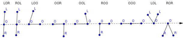
In order to create the locational code each octant gets a 3-bit number between 0 and 7 assigned, depending on the node’s relative position to it’s parent’s center. The possible relative positions are: bottom-left-front (000), bottom-right-front (001), bottom-left-back (010), bottom-right-back (011), top-left-front (100), top-right-front (101), top-left-back (110), top-right-back (111). The locational code of any child node in the tree can be computed recursively by concatenating the octant numbers of all the nodes from the root down to the node in question. The octant numbers are illustrated in the figure below.

The AABB of the node can be stored explicitly as before, or it can be computed from the node’s tree depth stored implicitly inside the locational code. To derive the tree depth at a node from its locational code a flag bit is required to indicate the end of the locational code. Without such a flag it wouldn’t be possible to distinguish e.g. between 001 and 000 001. By using a 1 bit to mark the end of the sequence 1 001 can be easily distinguished from 1 000 001. Using such a flag is equivalent to setting the locational code of the Octree root to 1. With one bit for the flag and three bits per Octree level, a 32-bit locational code can represent at maximum a tree depth of 10, a 64-bit locational code a tree depth of 21. Given the locational code of a node, its depth in the Octree can be computed as . An efficient implementation using bit scanning intrinsics is given below for GCC and Visual C++.

size_t Octree::GetNodeTreeDepth(const OctreeNode *node)
{
    assert(node->LocCode); // at least flag bit must be set
    // for (uint32_t lc=node->LocCode, depth=0; lc!=1; lc>>=3, depth++);
    // return depth;

#if defined(__GNUC__)
    return (31-__builtin_clz(node->LocCode))/3;
#elif defined(_MSC_VER)
    long msb;
    _BitScanReverse(&msb, node->LocCode);
    return msb/3;
#endif
}

When sorting the nodes by locational code the resulting order is the same as the pre-order traversal of the Octree, which in turn is equivalent to the Morton Code (also known as Z-Order Curve). The Morton Code linearly indexes multi-dimensional data, preserving data locality on multiple levels.

Tree traversal

Given the locational code, moving further down or up the Octree is a simple two-step operation consisting of (1) deriving the locational code of the next node and (2) looking-up the node in the hash-map.

For traversing up the Octree, first, the locational code of the parent node must be determined. This is done by removing the least significant three bits of the locational code of the current node. Now, the parent node can be retrieved by doing a hash map look-up with the previously computed locational code. An exemplary implementation is given below.

class Octree
{
public:
    OctreeNode * GetParentNode(OctreeNode *node)
    {
        const uint32_t locCodeParent = node->LocCode>>3;
        return LookupNode(locCodeParent);
    }

private:
    OctreeNode * LookupNode(uint32_t locCode)
    {
        const auto iter = Nodes.find(locCode);
        return (iter == Nodes.end() ? nullptr : &(*iter));
    }

private:
    std::unordered_map<uint32_t, OctreeNode> Nodes;
};

For traversing down the Octree, first, the locational code of the child in question must be computed. This is done by appending the octant number of the child to the current node’s locational code. After that the child node can be retrieved by doing a hash map look-up with the previously computed locational code. The following code visits all nodes of an Octree from the root down to the leafs.

void Octree::VisitAll(OctreeNode *node)
{
    for (int i=0; i<8; i++)
    {
        if (node->ChildExists&(1<<i))
        {
            const uint32_t locCodeChild = (node->LocCode<<3)|i;
            const auto *child = LookupNode(locCodeChild);
            VisitAll(child);
        }
    }
}

Full Octrees

In a full or complete Octree, every internal node has eight children and all leaf nodes have exactly the same tree depth which is fixed a priori. A full Octree has leaf nodes. Thus, it’s equal to a regular 3D grid with a resolution of . The total number of tree nodes can be computed as . Full Octrees of four successive subdivision levels are depicted in the figure below.

Thanks to the regularity of a full Octree it can be implemented without explicitly storing any tree structure and cell size information in the nodes. Hence, a single node consists solely of the pointer to the objects; which is eight bytes on a 64-bit machine. Similar to binary trees, full Octrees can be stored pointer-less in an array FullOctreeNode Nodes[K] (zero-based). The children of any node Nodes[i] can be found at Nodes[8*i+1] to Nodes[8*i+8], the parent of node Nodes[i] can be found at Nodes[floor((i-1)/8)] if i is not the root node ().

The most common application of full Octrees are non-sparse, static scenes with very evenly distributed geometry. If not most of the nodes contain objects, memory savings due to small node structs are quickly lost by the huge amount of nodes that need to be allocated. A full Octree of depth consists of (1.2 billion) nodes which consume around 9.14 GiB of memory.

Wrap up

Which node representation to choose for an Octree implementation depends mainly on the application. There are three major aspects that can help deciding on the representation.

1. How much data will supposedly be stored in the Octree? Is the reduced node size of an implicit node representation crucial for keeping the memory usage in check?
2. Will the Octree be subject to frequent changes? Pointer-based node representations are much more suitable for modifying Octrees than implicit node representations.
3. Will the Octree be sparsely or densely populated? How much memory can be saved by supporting on-demand allocation of nodes? Is maybe a full Octree suitable?

---

1. I. Gargantini. An Effective Way to Represent Octrees. Communications of the ACM, Volume 25 Issue 12, Dec. 1982, Pages 905-910 ↩

Advanced Octrees 1: preliminaries, insertion strategies and maximum tree depth

Introduction

An Octree is a recursive, axis-aligned, spatial partitioning data structure commonly used in computer graphics to optimize collision detection, nearest neighbor search, frustum culling and more. Conceptually, an Octree is a simple data structure. However, when digging deeper into the literature one will find many interesting, not very well-known techniques for optimizing and extending Octrees. This is why I decided to write a series of blog posts about Octree techniques not widely covered on the Internet. This series will consist of five posts covering the following topics:

1. Preliminaries, insertion strategies and maximum tree depth
2. Different node representations for memory footprint reduction
3. Non-static Octrees to support moving objects and expanding/shrinking Octrees
4. Loose Octrees for optimizing insertion and culling hotspots
5. Accessing a node’s neighbors

I’ll publish the posts of this series one by one during the next few weeks, starting today with the first one on preliminaries, insertion strategies and an upper bound for the maximum Octree depth. Thanks for reading!

Preliminaries

An Octree hierarchically subdivides a finite 3D volume into eight disjoint octants. In the following, octants are also called nodes in the context of tree data structures and cells in the context of space. An Octree’s root cell encloses the entire world. Sometimes, Octrees are introduced as subdividing space into cubes instead of arbitrarily sized boxes. Generally, arbitrarily sized boxes work equally well and there’s no need to adjust the root cell’s size to have the shape of a cube. However, cube-shaped cells slightly speed-up cell subdivision computations and the cell size can be stored as just one float per node instead of three. The general structure of an Octree is illustrated in the figure below.

An Octree is constructed by recursively subdividing space into eight cells until the remaining number of objects in each cell is below a pre-defined threshold, or a maximum tree depth is reached. Every cell is subdivided by three axis-aligned planes, which are usually placed in the middle of the parent node. Thus, each node can have up to eight children. The possibility not to allocate certain child nodes allows, in contrast to regular grids, to store sparsely populated worlds in Octrees.

Insertion strategies

Points are dimensionless and thereby have no spatial extent. Thus, if points are stored in an Octree, they can be unambiguously assigned to exactly one node. However, if objects with spatial extent like polygons are stored in an Octree, their midpoint can fall into a cell while the object it-self straddles the cell boundary. In that case there are basically three options.

1. The object in question is split along the boundaries of the straddling cells and each part is inserted into its corresponding cell. This approach has two disadvantages. First, the splitting operation might imply costly computations. Second, the data structures are more complicated, because the split-off objects need to be stored somewhere.

2. The object in question is added to each cell it straddles. This option is disadvantageous when the Octree needs to be updated, because it can contain duplicate references to the same object. Furthermore, the culling performance gets worse, because the same object might be found in more than one visible cell. Additionally, special care must be taken when subdividing cells. If after subdividing a cell all objects straddle the very same newly created sub-cell(s), all objects will be inserted again into the same sub-cell(s) causing yet another subdivision step. This results in an infinite loop, only stopped when the maximum tree depth is reached.

3. The object in question is stored in the smallest Octree cell it’s completely enclosed by. This option results in many unnecessary tests, because objects are stored in inner nodes instead of leaf nodes in case they straddle any child cell further down the tree.

In some of the following posts of this series I’ll come back to the different insertion strategies and show in which situation which of the strategies is advantageous. Especially, Loose Octrees are a particularly nice way of overcoming most of the downsides discussed above.

Maximum tree depth

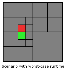
Let’s assume an Octree contains points. As described in the previous section, each of the points can only fall exactly into one node. Is it possible to establish a relation between the number of points and the maximum Octree depth ? It turns out, that the number of Octree nodes (=> the Octree depth) is not limited by the number of points. The reason is, that if the points are distributed closely enough in multiple widespread clusters, the number of Octree nodes can grow arbitrarily large. Look at the following figure for an illustration.

In order to split any of the two point clusters, the Octree must be subdivided a few times first. As the points inside the clusters can be arbitrarily close and the clusters can be arbitrarily far away from each other, the number of subdivision steps, and therefore the number of Octree nodes is not limited by the size of the point set. That shows that generally, Octrees cannot be balanced as we are used to from traditional tree data structures.

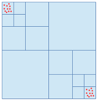
Nevertheless, we can come up with another upper bound for the maximum tree depth. Let’s assume a cubic Octree for simplicity. Given the minimum distance between any two points in the point set and the side length of the root cell , it can be shown that the maximum Octree depth is limited by . The following proof for this upper bound is rather simple.
The maximum distance between any two points in a cell at depth is given by . Any inner node encloses at least two points, otherwise it would be a leaf node. Hence, the maximum distance between any two points in this cell is guaranteed to be bigger than the minimum distance between any two points of the point set. Therefore, it holds that .

That’s it for today. Stay tuned for the next article!

On finding 1-bit sequences

Principles

Given is an arbitrary integer variable. How to find the index of the least significant bit (LSB) of the first 1-bit sequence of length >= n? Assuming n=4, let’s consider the following example of a random 32-bit integer value. The index we’re looking for is 10 in this case (indicated by the V character).

    31      24 | 23      16 | 15    V 8 | 7      0
MSB  01000111  |  11111101  |  10111100 | 01101001  LSB

Using a series of bit-wise and and shift-right operations the index of the LSB of the first 1111 sequence in the integer x can be found with the following trick.

x &= x>>1;
x &= x>>2;
index = __builtin_ffs(x)-1; // use _BitScanForward in Visual C++

After the first statement every 1 in x indicates the start of a 11 sequence. After the second statement every 1 in x indicates the start of a 1111 sequence. In the last statement the GCC intrinsic __builtin_ffs() (use _BitScanForward() if you’re on Visual C++) returns the bit position of the first set bit, starting from the LSB.
Note, that it doesn’t work to shift by four bits at once because it’s necessary to combine neighboring 1-bits to make sure that there are no 0-bits in-between. The following example illustrates how shifting by 3 bits wrongly yields two isolated 1-bits. In contrast, shifting by 2 bits correctly yields a sequence of 2 bits which can be further reduced into a single 1-bit indicating the start of the 1111 sequence.

 shift by 2    shift by 3
  01111010      01111010
& 00011110    & 00001111
= 00011010    = 00001010
    ok           wrong

Arbitrary sequence lengths

By cleverly choosing the number of bits to shift, it’s even possible to extend this construction to find bit sequences which length is not a power of two. As the order of the and-shift-right operations has no relevance, the following algorithm can be used to compute the number of bits to shift in order to find the n-bit sequence index. The sum of shifted bits must be equal to n-1 and the number of bits to shift is halved in each iteration. Therefore, the total number of executed iterations is ceil(log2(n)).

int FindBitSeqIndexLsb(int x, int n)
{
    assert(n >= 0 && n <= 32);

    while (n > 1)
    {
        const int shiftBits = n>>1;
        x &= (unsigned)x>>shiftBits; // shift in zeros from left
        n -= shiftBits;
    }

    return __builtin_ffs(x)-1; // use _BitScanForward in Visual C++
}

Exact sequence length

The described method finds bit sequences of length >= n. In case you’re looking for a bit sequence of exactly n bits, the following statement can be inserted right before the LSB scan is performed. This statement masks out any 1-bit which has a 1 on its left or right side. All the remaining 1-bits are isolated and indicate the start of a sequence of exactly n bits.

mask = (~(x<<1))&(~((unsigned)x>>1)); // shift in zeros from left and right
x &= mask;

Sequence alignment

To account for aligned bit sequences, unaligned 1-bits can be simply masked out from x before the LSB scan is performed. For example, to regard only bit sequences starting at nibble boundaries x can be modified with the operation x &= 0x11111111 (it is 0x...11 = 0b...00010001) to clear all bits not starting at an index which is a multiple of four.

Computing oriented minimum bounding boxes in 2D

Introduction

Oriented bounding boxes are an important tool for visibility testing and collision detection in computer graphics. In this post I want to talk about how to compute the oriented minimum bounding box (OMBB) of an arbitrary polygon in two dimensions. As a polygon just enforces an ordering on a set of points (vertices), everything described in the following equally applies to simple point sets. Minimum in this context refers to the area of the bounding box. A minimum oriented bounding box is also known as smallest-area enclosing rectangle. However, I will stick to the former term throughout this article as it is more frequently used in the computer graphics world.

The easiest way of computing a bounding box for a polygon is to determine the minimum and maximum – and – coordinates of its vertices. Such an axis aligned bounding box (AABB) can be computed trivially but it’s in most cases significantly bigger than the polygon’s OMBB. Finding the OMBB requires some more work as the bounding box’ area must be minimized, constrained by the location of the polygon’s vertices. Look at the following figure for an illustration (AABB in blue, OMBB in red).

The technique for computing OMBBs presented in the following consists of two detached steps. In the first step the convex hull of the input polygon is computed. If the polygon is convex this step can be omitted because a convex polygon is equal to its convex hull. In the second step the Rotating Calipers method is employed on the convex hull to compute the resulting OMBB. I will focus on the Rotating Calipers method because it’s not very widely known in comparison to the numerous ways of computing convex hulls.

Convex hulls

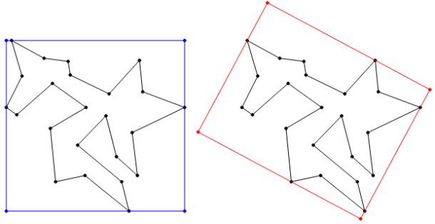
In less mathematical but more illustrative terms the convex hull of a set of points can be described as the closed polygonal chain of all outer points of the set, which entirely encloses all set elements. You can picture it as the shape of a rubber band stretched around all set elements. The convex hull of a set of two-dimensional points can be efficiently computed in . In the figure below the convex hull of the vertices of a concave polygon is depicted.

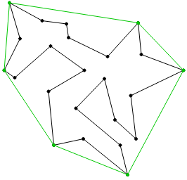
There are numerous algorithms for computing convex hulls: Quick Hull, Gift Wrapping (also known as Jarvis March), Graham’s Algorithm and some more. I’ve chosen the Gift Wrapping algorithm for my implementation because it’s easy to implement and provides good performance in case is small or the polygon’s convex hull contains only a few vertices. The runtime complexity is , where is the number of vertices in the convex hull. In the general case Gift Wrapping is outperformed by other algorithms. Especially, when all points are part of the convex hull. In that case the complexity degrades to .

As there are many good articles on the Gift Wrapping algorithm available online, I won’t describe it another time here. Instead I want to focus on the lesser-known Rotating Calipers method for computing OMBBs. However, take care that your convex hull algorithm correctly handles collinear points. If multiple points lie on a convex hull edge, only the spanning points should end up in the convex hull.

Rotating Calipers

Rotating Calipers is a versatile method for solving a number of problems from the field of computational geometry. It resembles the idea of rotating a dynamically adjustable caliper around the outside of a polygon’s convex hull. Originally, this method was invented to compute the diameter of convex polygons. Beyond that, it can be used to compute OMBBs, the minimum and maximum distance between two convex polygons, the intersection of convex polygons and many things more.

The idea of using the Rotating Calipers method for computing OMBBs is based on the following theorem, establishing a connection between the input polygon’s convex hull and the orientation of the resulting OMBB. The theorem was proven in 1975 by Freeman and Shapira¹:

The smallest-area enclosing rectangle of a polygon has a side collinear with one of the edges of its convex hull.

Thanks to this theorem the number of OMBB candidates is dramatically reduced to the number of convex hull edges. Thus, the complexity of the Rotating Calipers method is linear if the convex hull is already available. If it isn’t available the overall complexity is bound by the cost of computing the convex hull. An example of a set of OMBB candidates (red) for a convex hull (green) is depicted in the figure below. Note, that there are as many OMBB candidates as convex hull edges and each OMBB candidate has one side flush with one edge of the convex hull.

To determine the OMBB of a polygon, first, two orthogonally aligned pairs of parallel supporting lines through the convex hull’s extreme points are created. The intersection of the four lines forms a rectangle. Next, the lines are simultaneously rotated about their supporting points until one line coincides with an edge of the convex hull. Each time an edge coincides, the four lines form another rectangle / OMBB candidate. This process is repeated until each convex hull edge once coincided with one of the four caliper lines. The resulting OMBB is the OMBB candidate with the smallest area. The entire algorithm is outlined step by step below.

1. Compute the convex hull of the input polygon.
2. Find the the extreme points and of the convex hull.
3. Construct two vertical supporting lines at and and two horizontal ones at and .
4. Initialize the current minimum rectangle area .
5. Rotate the supporting lines until one coincides with an edge of the convex hull.
   1. Compute the area of the current rectangle.
   2. Update the minimum area and store the current rectangle if .
6. Repeat step 5 until all edges of the convex hull coincided once with one of the supporting lines.
7. Output the minimum area rectangle stored in step 5.2.

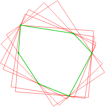
In practice, in every iteration the smallest angle between each caliper line and its associated, following convex hull edge is determined. Then, all caliper lines are rotated at once by and the associated convex hull edge of the caliper line enclosing the smallest angle is advanced to the next convex hull edge.

Wrap up

Rotating Calipers is a very elegant method for computing OMBBs in two dimensions. O’Rourke generalized it to three dimensions, yielding an algorithm of cubic runtime complexity. However, in practice approximation algorithms are used for three dimensional data because they’re usually faster. Beyond that, it's worth knowing the Rotating Calipers technique as it can be employed with minor changes to numerous other geometric problems. Depending on the programming language the implementation of the entire algorithm, including the convex hull computation, requires merely 150-200 lines of code. My sample implementation in Javascript can be found in my github repository.

---

1. H. Freeman, R. Shapira. Determining the minimum-area encasing rectangle for an arbitrary closed curve. Communications of the ACM, 18 Issue 7, July 1975, Pages 409-413 ↩

Optimizing binary search

Introduction

Binary search finds the index of a specified value (also called search key) in a pre-sorted array. Binary search is a very efficient and elegant algorithm which is used in a large number of data structures and algorithms. It has a runtime complexity of O(log N), where N is the number of elements to be searched through, because in each step the remaining number of array elements is halved.

Even though, the binary search algorithm is generally extremely fast I recently designed a data structure where the binary search was the major bottleneck. The said data structure performs successively a vast number of binary searches on a very large, static array of integers. The array can have a size of up to 100 billion unsigned 32-bit integers which corresponds to around 372.5 GB of raw data. To search for the first occurrence of an arbitrary key in an array of 100 billion elements a binary search touches floor(log2(N)+1)) = 30 elements, with N = 100000000000.

This is not an article about how to implement the binary search algorithm. More information on that can be found in plenty of resources online. The implementation of the optimization technique described in the rest of this post can be found in the accompanying github repository.

Memory hierarchy

Considering the size of the data set the first few array accesses are guaranteed to cause cache misses; or even worse page misses depending on the amount of available main memory. On machines with little main memory a page miss requires the operating system to fetch the corresponding block containing the required array element from disk (obviously this would require some additional code logic). Accessing main memory is roughly 200x slower than accessing the first level cache. The random access time of a modern SSD is typically under 0.1 ms, which is roughly 1000x slower than accessing main memory. The random access times of spinning disks vary considerably and are usually in the order of a few milliseconds. Assuming a random access time of 5 ms, accessing a spinning disk is roughly 50000x slower than accessing main memory. Take these numbers with a grain of salt. They are by no means accurate and will be considerably different measured on concrete systems. However, the overall orders of magnitude are correct and give an intuitive feeling of how costly array accesses can be.

Look-up tables

The previous paragraph should have cleared up why array accesses can be costly, especially when data is stored "far away" from the CPU. As a consequence it seems reasonable to try reducing the runtime costs of a binary search by reducing the number of array accesses needed for a search. This is a widely used optimization technique: an increased memory consumption is traded for increased performance.

The number of array accesses can be reduced by limiting the initial search range from left = 0, right = N-1 to anything smaller which is guaranteed to still contain the search key. The simple binary structure of unsigned integers allows us to use some of the high bits as an index into a look-up table (LUT) containing the reduced search range for the corresponding key. The more bits are used the bigger is the resulting speed-up, but the more memory is used. Using 16 bits requires only a 512 KB LUT. Using 24 bits requires already a 128 MB LUT. Let's consider exemplary a 16-bit LUT where the highest 16-bit of the search key are mapped. Each LUT entry maps to a sub-range in the value array that can contain up to 65536 different values.

0 [0x00000..0x0ffff] -> left = index of first element >= 0, right = index of last element < 65536
1 [0x10000..0x1ffff] -> left = index of first element >= 65536, right = index of last element < 131072
2 [0x20000..0x2ffff] -> left = index of first element >= 131072, right = index of last element < 196608
...

Let's consider a search for the key 114910 which is in hex 0x0001c0de. In order to obtain the LUT index for the key a right-shift by 16 bits is performed: lutIdx = key>>16, which results in lutIdx = 0x0001 = 1. The sub-range stored in the LUT at element 1 is guaranteed to contain all values in the range 65536 <= key < 131072. Following, the binary search, taking the search key, as well as the interval start and end as arguments, can be invoked by calling:

BinarySearch(key, Lut[lutIdx].left, Lut[lutIdx].right);

This is very little, simple and efficient code but how to populate the LUT? It turns out that populating the LUT can be done very efficiently in O(N) with a single, sequential pass over the input array. Even though, all elements must be touched once to populate the LUT, the sequential nature of the algorithm allows prefetching required data in advance and exploits the largely increased performance characteristics of spinning disks for sequential reads. The algorithm to populate the LUT is depicted in C++ below.

std::vector<std::pair<size_t, size_t>> Lut;

void InitLut(const std::vector<uint32_t> &vals, size_t lutBits)
{
    // pre-allocate memory for LUT
    const size_t lutSize = 1<<lutBits;
    const size_t shiftBits = 32-lutBits; // for 32-bit integers!
    Lut.resize(lutSize);

    // populate look-up-table
    size_t thresh = 0, last = 0;

    for (ssize_t i=0; i<(ssize_t)vals.size()-1; i++)
    {
        const size_t nextThresh = vals[i+1]>>shiftBits;
        Lut[thresh] = {last, i};

        if (nextThresh > thresh) // more than one LUT entry to fill?
        {
            last = i+1;
            for (size_t j=thresh+1; j<=nextThresh; j++)
                Lut[j] = {last, i+1};
        }

        thresh = nextThresh;
    }

    // set remaining thresholds that couldn't be found
    for (size_t i=thresh; i<Lut.size(); i++)
        Lut[i] = {last, vals.size()-1};
}

The LUT is implemented as an array of pairs. Each pair represents the interval the corresponding LUT entry maps to. To populate the LUT, the outer for-loop iterates over the pre-sorted array and calculates the number of LUT entries to fill between two successive array elements. The inner for-loop fills the LUT accordingly. As the start of each LUT entry can be derived from the end of the previous one, the last variable keeps track of the end of the last interval. The intervals are non-overlapping and it holds that the end of an interval is the beginning of the next interval minus one: Lut[i].second = Lut[i+1].first-1. As a consequence, the memory size of the LUT can be halved by storing only the interval starts and computing the interval ends as described. For simplicity reasons the depicted code is without this improvement, in contrast to the code in the accompanying github repository.

Other data types

The presented LUT-based optimization only works for data types that are compatible with a simple bit-wise comparison. This means that more significant bits must have a bigger influence on the value's magnitude than less significant bits. So do signed integers and floats work as well? As long as they're positive there are no problems, because for any two positive signed integers or floats x and y it holds that if x <= y it follows that UIR(x) <= UIR(y), where UIR() denotes the binary unsigned integer representation. However, negative values cause problems. Hence, when creating the LUT and when doing a range look-up the array elements and the search key must be mapped to an ordered range using a bijective mapping as described below.

Signed integers

Signed integers are stored in two's complement, in which the most significant bit (MSB) represents the sign: if the MSB is set the value is negative, otherwise it's positive. Therefore, signed integers compare greater using bit-wise comparison than unsigned ones. It turns out, that by simply flipping the sign bit the ordering can be fixed. It's important to note that flipping the sign bit is only enough if two's complement is used. If a simple signed magnitude representation is used negative values are not automatically reversed. In that case not only the sign bit but also all the remaining bits have to flipped when the sign bit is set. For clarity look at the following example of two's complement integers where FSB() denotes the function that flips the sign bit: FSB(-6 = 11111010) = 01111010 = 122 < FSB(-5 = 11111011) = 01111011 = 123 < FSB(2 = 00000010) = 10000010 = 130. In contrast, if a signed magnitude representation is used flipping the sign bit is not sufficient anymore as the following example illustrates: -6 < -5, however FSB(-6 = 10000110) = 00000110 = 6 > FSB(-5 = 10000101) = 00000101 = 5.

Floating point

Floating point values (I'm talking about IEEE 754) are a bit more nasty than signed integers. Their signed magnitude representation has exactly the same problem as signed magnitude represented integers have, outlined in the previous section. To overcome this problem all the remaining bits just have to be flipped as well if the sign bit was set. For further information read the article of Michael Herf about Radix Sort for floats on Stereopsis. One possible implementation in C++ is:

// taken from Michael Herf's article on Stereopsis
uint32_t MapFloat(float val)
{
    // 1) flip sign bit
    // 2) if sign bit was set flip all other bits as well
    const uint32_t cv = (uint32_t &)val;
    const uint32_t mask = (-(int32_t)(cv>>31))|0x80000000;
    return cv^mask;
}

Results

I analyzed the performance gain of the LUT optimization by searching 10 million times through an array of 1 billion 32-bit integers. The integers were uniformly distributed in the interval [0, 0xffffffff]. In each search a randomly determined key from the data set was used. The performance was measured on a laptop with a Core(TM) i7-3612QM CPU (Ivy Bridge) at 2.1 GHz with 6 MB L3 cache and 8 GB RAM. The results of the standard binary search and the LUT optimized binary search for different LUT sizes are depicted in the table below. The speed-up is related to C++ standard binary search function std::lower_bound(), not my own implementation used for the range reduced binary search.

Algorithm	LUT size	Time needed	Searches/second	Speed-up
std::lower_bound()	–	9.373 secs	1.07 m	–
LUT binary search	8-bit (2 KB)	8.592 secs	1.16 m	1.09x
LUT binary search	16-bit (512 KB)	3.873 secs	2.58 m	2.42x
LUT binary search	24-bit (128 MB)	1.99 secs	5.03 m	4.71x

The 16-bit LUT binary search is more than 2.5x, the 24-bit LUT binary search is even almost 5x faster than C++'s standard binary search implementation. The amount of required additional code is neglectable and the LUT memory size can be configured granularly by adjust the number of bits used to index the LUT. Thanks to the O(N) complexity of the LUT population algorithm the discussed optimization is even feasible in situations where the underlying value array changes from time to time. Especially, in situations where parts of the data set are only resident on hard disk the reduced number of array accesses saves a considerable amount of work. By using simple mappings the LUT optimization can be applied as well to signed integer and even floating point values. For a sample implementation checkout the accompanying github repository.