Advanced Octrees 4: finding neighbor nodes

Introduction

Welcome to part four of the the Advanced Octrees series. Here you can find part one, two and three. In this part I show you how to access neighbor nodes in Quadtrees. The algorithm can be naturally extended to Octrees, but it’s easier to understand and code in just two dimensions. Neighbors are such nodes that either share an edge in horizontal (west, east) or vertical (north, south) direction, or that share a vertex in one of the four diagonal directions (north-west, north-east, south-west, south-east). See the figure below for an illustration. The node of which we want to find the neighbors is colored green. In the following this node is called source node. The neighbor nodes are colored red and labeled with the corresponding direction.

In the literature Quadtree neighbor finding algorithms are distinguished by two properties:

1. Does the algorithm operate on pointer-based Quadtrees or on linear Quadtrees? Read up on different Quadtree representations in part two of this series. The algorithm discussed in this post is based on a pointer representation.
2. Can the algorithm only find neighbors of equal or greater size, or can it also find neighbors of smaller size. We’ll see later that finding neighbors of smaller size is somewhat harder. Greater / equal / smaller refers to the difference in tree level between the source node and the neighbor nodes.

The figure below shows examples of neighbor relationships in north direction between nodes on different tree levels. Note, that a node can have more than one neighbor per direction if the sub-tree on the other side of the north edge is deeper than the sub-tree of the source node.

Algorithm

The input to the algorithm is a direction and an arbitrary Quadtree node (inner of leaf). The output is a list of neighbor nodes in the given direction. The neighbors can be of greater size, equal size or smaller size (see previous figure). The algorithm is symmetric with respect to the direction. That’s why I only show an implementation for the north direction. It should be easy to extend the implementation to the other seven directions.

The neighbor finding happens in two steps. In step 1 we search for a neighbor node of greater or equal size (yellow). If such a node can be found we perform the second step, in which we traverse the sub-tree of the neighbor node found in step 1 to find all neighbors of smaller size. The two steps are illustrated in the figure below.

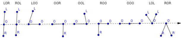
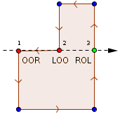
So how to find the neighbor of greater or equal size? Starting from the source node the algorithm traverses up the tree as long as the current node is not a south child of the parent, or the root is reached. After that the algorithm unrolls the recursion descending downwards always picking the south node. The node the recursion stops at is the north neighbor of the source node. This node is always on the same tree level as the source node, or further up the tree. Because the source node can be in the west or in the east, there’s a case distinction necessary to handle both possibilities.

Below is an implementation in Python. The code uses a pointer based Quadtree data structure, in which every node consists of a parent and four children. The children array is indexed using the constants NW, NE, SW and SE. The full code can be found on Github.

def get_neighbor_of_greater_or_equal_size(self, direction):   
  if direction == self.Direction.N:       
    if self.parent is None: # Reached root?
      return None
    if self.parent.children[self.Child.SW] == self: # Is 'self' SW child?
      return self.parent.children[self.Child.NW]
    if self.parent.children[self.Child.SE] == self: # Is 'self' SE child?
      return self.parent.children[self.Child.NE]

    node = self.parent.get_neighbor_of_greater_or_same_size(direction)
    if node is None or node.is_leaf():
      return node

    # 'self' is guaranteed to be a north child
    return (node.children[self.Child.SW]
            if self.parent.children[self.Child.NW] == self # Is 'self' NW child?
            else node.children[self.Child.SE])
  else:
    # TODO: implement symmetric to NORTH case

In step 2 we use the neighbor node obtained in step 1 to find neighbors of smaller size by recursively descending the tree in south direction until we reach the leaf nodes. On the way we always keep both, the south west and the south east node, because any node lower in the tree than the neighbor node from step 2 is smaller than the source node and therefore a neighbor candidate.

def find_neighbors_of_smaller_size(self, neighbor, direction):   
  candidates = [] if neighbor is None else [neighbor]
  neighbors = []

  if direction == self.Direction.N:
    while len(candidates) > 0:
      if candidates[0].is_leaf():
        neighbors.append(candidates[0])
      else:
        candidates.append(candidates[0].children[self.Child.SW])
        candidates.append(candidates[0].children[self.Child.SE])

      candidates.remove(candidates[0])

    return neighbors
  else:
    # TODO: implement other directions symmetric to NORTH case

Finally, we combine the functions from step 1 and 2 to get the complete neighbor finding function.

def get_neighbors(self, direction):   
  neighbor = self.get_neighbor_of_greater_or_equal_size(direction)
  neighbors = self.find_neighbors_of_smaller_size(neighbor, direction)
  return neighbors

Complexity

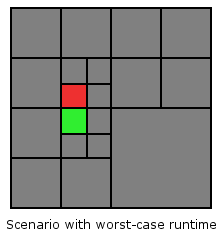
The complexity of this algorithm is bounded by the depth of the Quadtree. In the worst-case the source node and its neighbors are on the last tree level but their first common ancestor is only the root node. This is the case for any node that lies directly below/above or left/right of the line splitting the root node horizontally/vertically. See the following picture for an illustration.

Splitting an arbitrary polygon by a line

In this post I present an algorithm for splitting an arbitrary, simple polygon by a line. My implementation is based on ideas from the article Spatial Partitioning of a Polygon by a Plane by George Vanecek, published in the book Graphics Gems V. The intention behind this post is covering all the details which the original article omitted. All polygons are assumed to be oriented counter clockwise. You can find the full source code of my implementation in this github repository.

Introduction

Splitting a polygon by a line is very closely related to clipping a polygon against a clip region, like a rectangle or another polygon. Splitting a polygon is easier and at the same time harder than clipping a polygon. It’s easier because you only clip against a single line and it’s harder because the resulting polygons cannot simply be discarded. It turns out, that splitting convex polygons is a lot easier than splitting concave polygons. The reason is that splitting convex polygons results in at most two new polygons, whereas splitting concave polygons can result in arbitrary many new polygons. Look at the following figure for an illustration.

Coming up with a correct implementation for concave polygons is tricky, because there are many corner cases that must be considered. In the following, first, an algorithm for splitting convex polygons is outlined. Afterwards, the algorithm is extended to concave polygons.

Convex polygons

Splitting convex polygons is pretty simple. Essentially, one iterates over the polygon’s vertices, checks on which side of the split line they lie and adds them accordingly either to the left or the right result polygon. When an edge crosses the split line, additionally, the intersection point must be added to both result polygons. Special care must be taken when multiple successive vertices lie on the split line. In that case, due to the convexity property, the entire polygon lies either on the left-hand or on the right-hand side of the polygon. When for the second time a polygon edge crosses the split line, we know that the first half of the polygon is already completely split off.

Concave polygons

In contrast to splitting convex polygons it requires some more algorithmic effort to split concave polygons. When the split line crosses a concave polygon for the second time, it doesn’t necessarily mean that the first half of the polygon is now completely split off. On the contrary, it might be that another new polygon to be split off just opened. To account for that, first, I tried to iterate over the polygon edges while carrying along a stack of open polygons. Whenever, I came across a vertex which belonged to the open polygon on the top of the stack I knew it just closed. This approach worked out well until I tried accounting for all the corner cases. Finally, I decided to use the method from the article mentioned in the introduction.

Idea of the algorithm

The intersection points between the split line and the polygon are key to the splitting algorithm. By pairing up 2-tuples of intersection points along the split line, the edges closing the result polygons can be determined. Conceptually, every two intersection points along the split line form a pair of edges, each closing one side of two neighboring result polygons. In a perfect world, the intersection points could be easily paired up after sorting them along the split line, relative to the split line’s starting point (cf. the left figure below). Unfortunately, in the real world special care must be taken when the split line doesn’t cross a polygon edge in middle, but only touches the start and/or end vertex. In such cases the pairing up of source points (red) and destination points (green) along the split line gets trickier (cf. the figure in the middle blow). As you can see, only certain intersection points qualify as sources and destinations and some intersection points even qualify as both (yellow, cf. the right figure below). Luckily, it’s possible to account for all of these cases as we’ll see later.

Computing the intersection points

To ease the splitting process it’s helpful to represent the polygon as a doubly linked list. We compute the intersection points between the split line and the polygon by iterating over each polygon edge e and determining on which side of the split line the edge’s start vertex e.Start and end vertex e.End lies. If e.Start lies on the split line e is added to the array EdgesOnLine, which contains all edges starting on the split line. If e.Start and e.End lie on opposite sides of the split line, a new edge starting at the intersection point is inserted into the polygon and added to EdgesOnLine. The edges in this array are of interest, because they start at the intersection points with the split line. The algorithm is outlined below.

for (auto &e : poly)
{
    const LineSide sideStart = GetLineSide(SplitLine, e.Start);
    const LineSide sideEnd = GetLineSide(SplitLine, e.End);

    if (sideStart == LineSide::On)
    {
        EdgesOnLine.push_back(e);
    }
    else if (sideStart != sideEnd && sideEnd != LineSide::On)
    {
        Point2 ip = IntersectLines(SplitLine, e);
        Edge *newEdge = poly.InsertEdge(e, ip);
        EdgesOnLine.push_back(newEdge);
    }
}

Sorting the intersection points

After all polygon edges have been intersected with the split line, the edges in the EdgesOnLine array are sorted along the split line by the distance between their starting points and the starting point of the split line. Sorting the EdgesOnLine array is crucial for pairing up the source and the destination edges by simply iterating over the array as we see in the following section.

std::sort(EdgesOnLine.begin(), EdgesOnLine.end(), [&](PolyEdge *e0, PolyEdge *e1)
{
    return (CalcSignedDistance(line, e0->StartPos) <
            CalcSignedDistance(line, e1->StartPos));
});

As Glenn Burkhardt pointed out in a comment, the Euclidean distance cannot be used as distance metric because it’s unsigned. The Euclidean distance can only be used as long as the split line’s starting point lies outside the polygon. In that case all points are on the same side of the split line’s starting point and the Euclidean distance provides a strict order along the split line. However, if the split line’s starting point is inside the polygon, points on two different sides of the split line’s starting point will both have positive distances, which can result in wrong sort orders. A formula for computing the signed Euclidean distance between two points can be derived from the formula for scalar projections. In case of co-linear lines (angle between the two vectors is |1|) the result equals the signed distance along the split line.

static double CalcSignedDistance(const QLineF &line, const QPointF &p)
{
    return (p.x()-line.p1().x())*(line.p2().x()-line.p1().x())+
           (p.y()-line.p1().y())*(line.p2().y()-line.p1().y());
}

Pairing up edges

As we’ve seen before, all edges in the EdgesOnLine array are either source edges, destination edges or both. The edges must be classified accordingly, in order to be able to determine between which pairs of edges a bridge must be created to split the polygon. The source/destination classification is the most important part of the algorithm and the hardest to get right due to plenty of corner cases.

The starting point e.Start of any edge e in the EdgesOnLine array lies on the split line. Each edge e has a predecessor edge e.Prev and a successor edge e.Next. They can lie either on the left-hand side (L), on the right-hand side (R) or on the split line (O). Hence, there’s a total of nine configuration possibilities that must be evaluated in order to find out if an edge is a source, a destination or both. All nine configurations are depicted in the figure below. The vertex order is shown in the caption of each configuration.

I simply examined examples to classify each configuration as source, destination or both. The configurations’ winding orders are key for the classification. Imagine to move along the split line from its starting point to its endpoint. The winding order at the current intersection point indicates if we’re currently inside the polygon or not. Let’s take exemplary the LOR and ROL cases. The LOR case is only encountered when transitioning from the outside to the inside of a polygon. Hence, it’s a source configuration. In contrast, the ROL case is only encountered when transitioning from the inside of the polygon to the outside. Hence, it’s a destination configuration. Below are sample polygons depicted for the classification of each source and each destination configuration.

It follows that LOR, ROR, LOL, OOR and LOO are source configurations and ROL, ROR, LOL, ROO and OOL are destination configurations. Note, that these two sets are not disjoint: ROR and LOL are source and destination configurations. However, these two configurations can only be sources if they have served as destinations before!
Another corner case occurs when two successive edge starting points lie on the split line. Look at the example depicted in the figure below. There are two source edges (red) of which the second one must be used as source, even though it comes second in the EdgesOnLine array.

The EdgesOnLine array contains three edges: two source edges (red) and one destination edge (green). When splitting the polygon it’s crucial to pair up the the second and the third edge, not the first and the third. So how do we figure out which source edge to select when iterating over the EdgesOnLine array? It turns out that the distance between the starting points of the two successive source edges in question and the starting point of the split line can be used. An OOR and LOO source edge is only selected if the following candidate edge isn’t further away from the start of the split line and therefore closer to the next destination.

Rewiring the polygon

After we’ve figured out how the classification of source and destination edges works, we can finally formulate the algorithm to split concave polygons. All we need to do is to iterate over the EdgesOnLine array while pairing up source and destination edges. Each pair denotes one side of the polygon that has to be be split off. At this point it pays off that we use a linked list representation for the polygon. The current polygon side is split off by inserting two new edges between the source and the destination edge. Therefore, we iterate over the EdgesOnLine array, obtain the next source and the next destination edge and insert two new, oppositely oriented edges between them. This bridging operation is depicted in the following figure.

The main loop of the rewiring process is depicted below. For reasons of brevity only the overall structure is shown. For more details look into the full implementation in the github repository.

for (size_t i=0; i<EdgesOnLine.size(); i++)
{
    // find source edge
    PolyEdge *srcEdge = useSrc;

    for (; !srcEdge && i<EdgesOnLine.size(); i++)
    {
        // test conditions if current edge is a source
    }

    // find destination edge
    PolyEdge *dstEdge = nullptr;

    for (; !dstEdge && i<EdgesOnLine.size(); )
    {
        // test conditions if current edge is a destination
    }

    // bridge source and destination edges
    if (srcEdge && dstEdge)
        CreateBridge(srcEdge, dstEdge);
}

Collecting the result polygons

The final step, after all bridge edges have been inserted, is collecting the resulting polygons. For that purpose I use the Visited attribute in the edge data structure to indicate if an edge has been visited already and therefore, has been assigned already to one of the result polygons.

Advanced Octrees 3: non-static Octrees

Welcome to the third part of the Advanced Octrees series. Make sure you’ve also read part one and two. Typically, Octrees are constructed once for geometry which is known a priori and doesn’t change anymore (e.g. the level in a computer game). However, there are applications where objects are moving through the world, or objects located outside the Octree’s root cell must be inserted after the Octree has been constructed already. One approach would be to simply reconstruct the entire Octree from scratch each time it’s modified. While working, obviously, this turns very inefficient as soon as the Octree contains more than just a handful objects. In this post I present a way to relocate moving objects in already constructed Octrees, as well as a way to expand/shrink Octrees.

Relocate moving objects

An Octree which contains moving objects must be updated whenever a moving object starts straddling its parent cell’s bounding box. Usually, the number of moving objects is considerably smaller than the number of static objects. Thus, it can be advantageous to maintain two Octrees: one containing all static and one containing all moving objects. Instead of reconstructing the Octree from scratch, it’s much faster to relocate only the objects that have moved out of their parent cell.

Duplicating objects straddling cell boundaries works great for static scenes. However, in dynamic scenes keeping track of multiple references to the same object contained in multiple different nodes adds unnecessary complexity. Therefore, it’s better to place objects in the lowest Octree cell which completely encloses the object (see part one). That way a minimum amount of pointer information must be updated when a moving object transitions from one cell into another.

To update an Octree with moving objects, first, a list of all objects that have moved out of their parent cell is obtained. Each object in this list is pushed up the Octree until it ends up in a node which completely encloses it. The object must remain in this node, as long as it straddles any child cell’s bounding box of its new parent. However, when the object keeps on moving into the same direction, there will be the moment it’s again completely enclosed by one of its parent’s child cells. Therefore, finally, all previously pushed up objects are tried to be moved down the Octree again, in order to place them in the smallest enclosing cell possible.
It can happen that objects move out of the Octree’s root cell. In that case the Octree must be expanded as described in the following section. It can also happen that after pushing a moving object up the Octree, the former parent node and all its child nodes remain empty. In that case the former parent node and its children can be safely removed.

Expanding and shrinking

The final extent of the world isn’t always known at the time the Octree is constructed. Consider a space game in which world entities can spawn at arbitrary locations, or where space ships can move around freely until they leave the Octree’s root cell. To handle such situations an Octree must be expanded and shrunk dynamically as game entities spawn, disappear or move.

Octrees can be expanded by allocating a new root node with seven new child nodes and the 8th child node being the old root node. It’s crucial to expand the Octree into the direction of the outlying object. Therefore, the center of the new root node must be chosen in such a way, that the outlying object falls into it, or that at least the distance between the outlying object and the new Octree root node decreases. This operation is repeated recursively until the outlying object finally falls into the Octree’s root cell. As the Octree’s extent grows exponentially (it doubles each tree level) any reasonably far away object will be enclosed after a few expansion steps.
To shrink an Octree the reverse operation can be applied. If seven out of eight root node children are empty, all seven children can be removed from the Octree and the remaining child becomes the Octree’s new root node.

Creating and deleting nodes at the top of hashed Octrees is very costly, because the locational code of all nodes below the new root node gets 3 bits longer and must be updated. Consequently, the hash map must be updated as well. If expanding/shrinking are rare operations it might be still worth using hashed Octrees. Though, usually, pointer-based implementations perform much better. For more information read part two.

Advanced Octrees 2: node representations

Introduction

Welcome to the second installment of the Advanced Octrees series. Make sure you’ve also read part one. In the second part I discuss different Octree data structure layouts. Essentially, literature distinguishes between two different layouts: the traditional layout using a pointer-based node representation and the implicit layout using an index-based node representation. Both layouts have their strong points and their weak points. Pointer-based node representations are advantageous if the Octree needs to be updated frequently and if memory consumption is not an issue. Implicit node representations pay off in memory limited applications.

Regardless of the chosen representation, the node struct always contains a pointer to the list of objects it encloses. Additionally, almost always the cell’s axis-aligned bounding box (AABB) is stored inside the node. The AABB can be stored in two different ways: either as two vectors AabbMin and AabbMax containing the AABB’s minimum and maximum corners, or as two vectors Center and HalfSize containing the AABB’s center and extent. If the Octree is cubic, all AABB sides have the same length and the storage size of the latter AABB representation can be reduced by storing HalfSize as a single float. Speedwise the center-extent representation is advantageous in most calculations (e.g. for view-frustum culling). Instead of storing the AABB inside the node, it can be recomputed while traversing the Octree. This is a memory consumption vs. compute trade-off.

All struct sizes given in the remainder of this post assume 64-bit wide pointers and the Vector3 class consisting of three 32-bit float variables. Let’s start with looking at pointer-based node representations first.

Pointer-based node representations

Standard representation

The most intuitive, pointer-based node representation consists of eight pointers to each of the eight child nodes. This representation supports on-demand allocation of nodes. On-demand allocation only allocates memory for child nodes, once an object is encountered which falls into the respective sub-cell. Some Octree implementations add pointers to the parent node for bottom-up traversals.

// standard representation (104 bytes)
struct OctreeNode
{
    OctreeNode * Children[8];
    OctreeNode * Parent; // optional
    Object *     Objects;
    Vector3      Center;
    Vector3      HalfSize;
};

As leaf nodes have no children, they don’t need to store child pointers. Therefore, two different node types, one for inner nodes and one for leaf nodes, can be used. To distinguish between inner nodes and leaf nodes, a flag must be stored additionally. The flag can be either stored as an additional bool variable IsLeaf, or encoded in the least significant bit of one of the pointers if the nodes are allocated with appropriate alignment (C++’s new operator usually aligns object types to the size of their largest member).

// inner node (105 bytes)                   // leaf node (41 bytes)
struct OctreeInnerNode                      struct OctreeLeafNode
{                                           {
    OctreeInnerNode * Children[8];              // leaf has no children
    OctreeInnerNode * Parent;                   OctreeInnerNode * Parent; // optional
    Object *          FirstObj;                 Object *          Objects;
    Vector3           Center;                   Vector3           Center;
    Vector3           HalfSize;                 Vector3           HalfSize;
    bool              IsLeaf;                   bool              IsLeaf;
};                                          };

Using two different node types, one for inner nodes and one for leaf nodes, can be applied as well to the following two representations.

Block representation

A significant amount of memory can be saved by storing just one pointer to a block of eight children, instead of eight pointers to eight children. That way the storage size of an inner node can be reduced from 105 bytes down to 49 bytes, which is only 47% of the original size. However, when a leaf node is subdivided always all eight children must be allocated. It’s not possible anymore to allocate child nodes on-demand, once the first object falling into the octant in question is encountered. Look at the following figure for an illustration of the block representation.

The corresponding code for the node struct is:

// block representation (49 bytes)
struct OctreeNode
{
    OctreeNode * Children;
    OctreeNode * Parent; // optional
    Object *     FirstObj;
    Vector3      Center;
    Vector3      HalfSize;
    bool         IsLeaf;
};

Sibling-child representation

On-demand allocation can reduce the amount of required memory for nodes significantly if the world is sparsely populated and thereby, many octants contain no objects. A trade-off between the standard representation and the block representation is the so called sibling-child representation. This representation allows on-demand allocation while storing only two node pointers per node instead of eight. The first pointer is NextSibling, which points to the next child node of the node’s parent. The second pointer is FirstChild, which points to the node’s first child node. Look at the following figure for an illustration of the sibling-child representation. Compare the number of required pointers per node to the standard representation.

In comparison to the standard representation, the sibling-child representation needs only 25% of the memory for pointers (two instead of eight pointers). As long as the child nodes are accessed sequentially the two representations perform equally well. However, accessing nodes randomly requires dereferencing on average four times more pointers. The code for the node struct is given below.

// sibling-child representation (56 bytes)
struct OctreeNode
{
    OctreeNode * NextSibling;
    OctreeNode * FirstChild;
    OctreeNode * Parent; // optional
    Object *     FirstObj;
    Vector3      Center;
    Vector3      HalfSize;
};

Comparison

The choice of the right pointer-based representation depends mainly on the importance of memory usage vs. traversal speed. Explicitly storing all eight child pointers wastes memory but makes traversing and modifying the Octree easy to implement and fast. In contrast, the sibling-child representation saves 50% memory as a single node is only 48 bytes instead of 92 bytes. However, the additional pointer indirections might complicate the traversal code and make it slower. It can be a good trade-off to store just a single pointer to a block of eight sub-cells. This representation needs only 40 bytes of memory per node and the traversal code is as easy as in the representation with eight child pointers. However, always allocating all eight sub-cells can waste memory in sparsely populated worlds with many empty sub-cells.

Implicit node representations

Linear (hashed) Octrees

Linear Octrees [Gargantini, 1982]¹, originally proposed for Quadtrees, combine the advantages of pointer-based and pointer-less representations. Linear Octrees provide easy and efficient access to parent and child nodes, even though no explicit tree structure information must be stored per node.

Overview

Instead of child and parent pointers, Linear Octrees store a unique index called locational code in each node. Additionally, all Octree nodes are stored in a hash map which allows directly accessing any node based on its locational code. The locational code is constructed in such a way, that deriving the locational codes for any node’s parent and children based on its own locational code is feasible and fast. To avoid unnecessary hash map look-ups for children which don’t exist, the node struct can be extended by a bit-mask indicating which children have been allocated and which haven’t.

struct OctreeNode // 13 bytes
{
    Object *    Objects;
    uint32_t    LocCode;     // or 64-bit, depends on max. required tree depth
    uint8_t     ChildExists; // optional
};

The locational code

In order to create the locational code each octant gets a 3-bit number between 0 and 7 assigned, depending on the node’s relative position to it’s parent’s center. The possible relative positions are: bottom-left-front (000), bottom-right-front (001), bottom-left-back (010), bottom-right-back (011), top-left-front (100), top-right-front (101), top-left-back (110), top-right-back (111). The locational code of any child node in the tree can be computed recursively by concatenating the octant numbers of all the nodes from the root down to the node in question. The octant numbers are illustrated in the figure below.

The AABB of the node can be stored explicitly as before, or it can be computed from the node’s tree depth stored implicitly inside the locational code. To derive the tree depth at a node from its locational code a flag bit is required to indicate the end of the locational code. Without such a flag it wouldn’t be possible to distinguish e.g. between 001 and 000 001. By using a 1 bit to mark the end of the sequence 1 001 can be easily distinguished from 1 000 001. Using such a flag is equivalent to setting the locational code of the Octree root to 1. With one bit for the flag and three bits per Octree level, a 32-bit locational code can represent at maximum a tree depth of 10, a 64-bit locational code a tree depth of 21. Given the locational code of a node, its depth in the Octree can be computed as . An efficient implementation using bit scanning intrinsics is given below for GCC and Visual C++.

size_t Octree::GetNodeTreeDepth(const OctreeNode *node)
{
    assert(node->LocCode); // at least flag bit must be set
    // for (uint32_t lc=node->LocCode, depth=0; lc!=1; lc>>=3, depth++);
    // return depth;

#if defined(__GNUC__)
    return (31-__builtin_clz(node->LocCode))/3;
#elif defined(_MSC_VER)
    long msb;
    _BitScanReverse(&msb, node->LocCode);
    return msb/3;
#endif
}

When sorting the nodes by locational code the resulting order is the same as the pre-order traversal of the Octree, which in turn is equivalent to the Morton Code (also known as Z-Order Curve). The Morton Code linearly indexes multi-dimensional data, preserving data locality on multiple levels.

Tree traversal

Given the locational code, moving further down or up the Octree is a simple two-step operation consisting of (1) deriving the locational code of the next node and (2) looking-up the node in the hash-map.

For traversing up the Octree, first, the locational code of the parent node must be determined. This is done by removing the least significant three bits of the locational code of the current node. Now, the parent node can be retrieved by doing a hash map look-up with the previously computed locational code. An exemplary implementation is given below.

class Octree
{
public:
    OctreeNode * GetParentNode(OctreeNode *node)
    {
        const uint32_t locCodeParent = node->LocCode>>3;
        return LookupNode(locCodeParent);
    }

private:
    OctreeNode * LookupNode(uint32_t locCode)
    {
        const auto iter = Nodes.find(locCode);
        return (iter == Nodes.end() ? nullptr : &(*iter));
    }

private:
    std::unordered_map<uint32_t, OctreeNode> Nodes;
};

For traversing down the Octree, first, the locational code of the child in question must be computed. This is done by appending the octant number of the child to the current node’s locational code. After that the child node can be retrieved by doing a hash map look-up with the previously computed locational code. The following code visits all nodes of an Octree from the root down to the leafs.

void Octree::VisitAll(OctreeNode *node)
{
    for (int i=0; i<8; i++)
    {
        if (node->ChildExists&(1<<i))
        {
            const uint32_t locCodeChild = (node->LocCode<<3)|i;
            const auto *child = LookupNode(locCodeChild);
            VisitAll(child);
        }
    }
}

Full Octrees

In a full or complete Octree, every internal node has eight children and all leaf nodes have exactly the same tree depth which is fixed a priori. A full Octree has leaf nodes. Thus, it’s equal to a regular 3D grid with a resolution of . The total number of tree nodes can be computed as . Full Octrees of four successive subdivision levels are depicted in the figure below.

Thanks to the regularity of a full Octree it can be implemented without explicitly storing any tree structure and cell size information in the nodes. Hence, a single node consists solely of the pointer to the objects; which is eight bytes on a 64-bit machine. Similar to binary trees, full Octrees can be stored pointer-less in an array FullOctreeNode Nodes[K] (zero-based). The children of any node Nodes[i] can be found at Nodes[8*i+1] to Nodes[8*i+8], the parent of node Nodes[i] can be found at Nodes[floor((i-1)/8)] if i is not the root node ().

The most common application of full Octrees are non-sparse, static scenes with very evenly distributed geometry. If not most of the nodes contain objects, memory savings due to small node structs are quickly lost by the huge amount of nodes that need to be allocated. A full Octree of depth consists of (1.2 billion) nodes which consume around 9.14 GiB of memory.

Wrap up

Which node representation to choose for an Octree implementation depends mainly on the application. There are three major aspects that can help deciding on the representation.

1. How much data will supposedly be stored in the Octree? Is the reduced node size of an implicit node representation crucial for keeping the memory usage in check?
2. Will the Octree be subject to frequent changes? Pointer-based node representations are much more suitable for modifying Octrees than implicit node representations.
3. Will the Octree be sparsely or densely populated? How much memory can be saved by supporting on-demand allocation of nodes? Is maybe a full Octree suitable?

---

1. I. Gargantini. An Effective Way to Represent Octrees. Communications of the ACM, Volume 25 Issue 12, Dec. 1982, Pages 905-910 ↩

Advanced Octrees 1: preliminaries, insertion strategies and maximum tree depth

Introduction

An Octree is a recursive, axis-aligned, spatial partitioning data structure commonly used in computer graphics to optimize collision detection, nearest neighbor search, frustum culling and more. Conceptually, an Octree is a simple data structure. However, when digging deeper into the literature one will find many interesting, not very well-known techniques for optimizing and extending Octrees. This is why I decided to write a series of blog posts about Octree techniques not widely covered on the Internet. This series will consist of five posts covering the following topics:

1. Preliminaries, insertion strategies and maximum tree depth
2. Different node representations for memory footprint reduction
3. Non-static Octrees to support moving objects and expanding/shrinking Octrees
4. Loose Octrees for optimizing insertion and culling hotspots
5. Accessing a node’s neighbors

I’ll publish the posts of this series one by one during the next few weeks, starting today with the first one on preliminaries, insertion strategies and an upper bound for the maximum Octree depth. Thanks for reading!

Preliminaries

An Octree hierarchically subdivides a finite 3D volume into eight disjoint octants. In the following, octants are also called nodes in the context of tree data structures and cells in the context of space. An Octree’s root cell encloses the entire world. Sometimes, Octrees are introduced as subdividing space into cubes instead of arbitrarily sized boxes. Generally, arbitrarily sized boxes work equally well and there’s no need to adjust the root cell’s size to have the shape of a cube. However, cube-shaped cells slightly speed-up cell subdivision computations and the cell size can be stored as just one float per node instead of three. The general structure of an Octree is illustrated in the figure below.

An Octree is constructed by recursively subdividing space into eight cells until the remaining number of objects in each cell is below a pre-defined threshold, or a maximum tree depth is reached. Every cell is subdivided by three axis-aligned planes, which are usually placed in the middle of the parent node. Thus, each node can have up to eight children. The possibility not to allocate certain child nodes allows, in contrast to regular grids, to store sparsely populated worlds in Octrees.

Insertion strategies

Points are dimensionless and thereby have no spatial extent. Thus, if points are stored in an Octree, they can be unambiguously assigned to exactly one node. However, if objects with spatial extent like polygons are stored in an Octree, their midpoint can fall into a cell while the object it-self straddles the cell boundary. In that case there are basically three options.

1. The object in question is split along the boundaries of the straddling cells and each part is inserted into its corresponding cell. This approach has two disadvantages. First, the splitting operation might imply costly computations. Second, the data structures are more complicated, because the split-off objects need to be stored somewhere.

2. The object in question is added to each cell it straddles. This option is disadvantageous when the Octree needs to be updated, because it can contain duplicate references to the same object. Furthermore, the culling performance gets worse, because the same object might be found in more than one visible cell. Additionally, special care must be taken when subdividing cells. If after subdividing a cell all objects straddle the very same newly created sub-cell(s), all objects will be inserted again into the same sub-cell(s) causing yet another subdivision step. This results in an infinite loop, only stopped when the maximum tree depth is reached.

3. The object in question is stored in the smallest Octree cell it’s completely enclosed by. This option results in many unnecessary tests, because objects are stored in inner nodes instead of leaf nodes in case they straddle any child cell further down the tree.

In some of the following posts of this series I’ll come back to the different insertion strategies and show in which situation which of the strategies is advantageous. Especially, Loose Octrees are a particularly nice way of overcoming most of the downsides discussed above.

Maximum tree depth

Let’s assume an Octree contains points. As described in the previous section, each of the points can only fall exactly into one node. Is it possible to establish a relation between the number of points and the maximum Octree depth ? It turns out, that the number of Octree nodes (=> the Octree depth) is not limited by the number of points. The reason is, that if the points are distributed closely enough in multiple widespread clusters, the number of Octree nodes can grow arbitrarily large. Look at the following figure for an illustration.

In order to split any of the two point clusters, the Octree must be subdivided a few times first. As the points inside the clusters can be arbitrarily close and the clusters can be arbitrarily far away from each other, the number of subdivision steps, and therefore the number of Octree nodes is not limited by the size of the point set. That shows that generally, Octrees cannot be balanced as we are used to from traditional tree data structures.

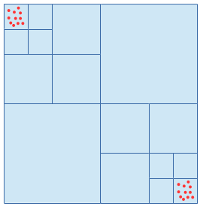
Nevertheless, we can come up with another upper bound for the maximum tree depth. Let’s assume a cubic Octree for simplicity. Given the minimum distance between any two points in the point set and the side length of the root cell , it can be shown that the maximum Octree depth is limited by . The following proof for this upper bound is rather simple.
The maximum distance between any two points in a cell at depth is given by . Any inner node encloses at least two points, otherwise it would be a leaf node. Hence, the maximum distance between any two points in this cell is guaranteed to be bigger than the minimum distance between any two points of the point set. Therefore, it holds that .

That’s it for today. Stay tuned for the next article!

Computing oriented minimum bounding boxes in 2D

Introduction

Oriented bounding boxes are an important tool for visibility testing and collision detection in computer graphics. In this post I want to talk about how to compute the oriented minimum bounding box (OMBB) of an arbitrary polygon in two dimensions. As a polygon just enforces an ordering on a set of points (vertices), everything described in the following equally applies to simple point sets. Minimum in this context refers to the area of the bounding box. A minimum oriented bounding box is also known as smallest-area enclosing rectangle. However, I will stick to the former term throughout this article as it is more frequently used in the computer graphics world.

The easiest way of computing a bounding box for a polygon is to determine the minimum and maximum – and – coordinates of its vertices. Such an axis aligned bounding box (AABB) can be computed trivially but it’s in most cases significantly bigger than the polygon’s OMBB. Finding the OMBB requires some more work as the bounding box’ area must be minimized, constrained by the location of the polygon’s vertices. Look at the following figure for an illustration (AABB in blue, OMBB in red).

The technique for computing OMBBs presented in the following consists of two detached steps. In the first step the convex hull of the input polygon is computed. If the polygon is convex this step can be omitted because a convex polygon is equal to its convex hull. In the second step the Rotating Calipers method is employed on the convex hull to compute the resulting OMBB. I will focus on the Rotating Calipers method because it’s not very widely known in comparison to the numerous ways of computing convex hulls.

Convex hulls

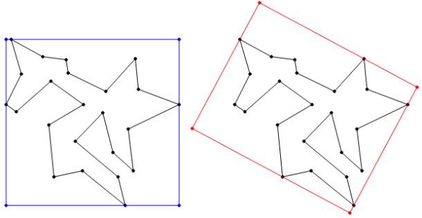
In less mathematical but more illustrative terms the convex hull of a set of points can be described as the closed polygonal chain of all outer points of the set, which entirely encloses all set elements. You can picture it as the shape of a rubber band stretched around all set elements. The convex hull of a set of two-dimensional points can be efficiently computed in . In the figure below the convex hull of the vertices of a concave polygon is depicted.

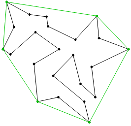
There are numerous algorithms for computing convex hulls: Quick Hull, Gift Wrapping (also known as Jarvis March), Graham’s Algorithm and some more. I’ve chosen the Gift Wrapping algorithm for my implementation because it’s easy to implement and provides good performance in case is small or the polygon’s convex hull contains only a few vertices. The runtime complexity is , where is the number of vertices in the convex hull. In the general case Gift Wrapping is outperformed by other algorithms. Especially, when all points are part of the convex hull. In that case the complexity degrades to .

As there are many good articles on the Gift Wrapping algorithm available online, I won’t describe it another time here. Instead I want to focus on the lesser-known Rotating Calipers method for computing OMBBs. However, take care that your convex hull algorithm correctly handles collinear points. If multiple points lie on a convex hull edge, only the spanning points should end up in the convex hull.

Rotating Calipers

Rotating Calipers is a versatile method for solving a number of problems from the field of computational geometry. It resembles the idea of rotating a dynamically adjustable caliper around the outside of a polygon’s convex hull. Originally, this method was invented to compute the diameter of convex polygons. Beyond that, it can be used to compute OMBBs, the minimum and maximum distance between two convex polygons, the intersection of convex polygons and many things more.

The idea of using the Rotating Calipers method for computing OMBBs is based on the following theorem, establishing a connection between the input polygon’s convex hull and the orientation of the resulting OMBB. The theorem was proven in 1975 by Freeman and Shapira¹:

The smallest-area enclosing rectangle of a polygon has a side collinear with one of the edges of its convex hull.

Thanks to this theorem the number of OMBB candidates is dramatically reduced to the number of convex hull edges. Thus, the complexity of the Rotating Calipers method is linear if the convex hull is already available. If it isn’t available the overall complexity is bound by the cost of computing the convex hull. An example of a set of OMBB candidates (red) for a convex hull (green) is depicted in the figure below. Note, that there are as many OMBB candidates as convex hull edges and each OMBB candidate has one side flush with one edge of the convex hull.

To determine the OMBB of a polygon, first, two orthogonally aligned pairs of parallel supporting lines through the convex hull’s extreme points are created. The intersection of the four lines forms a rectangle. Next, the lines are simultaneously rotated about their supporting points until one line coincides with an edge of the convex hull. Each time an edge coincides, the four lines form another rectangle / OMBB candidate. This process is repeated until each convex hull edge once coincided with one of the four caliper lines. The resulting OMBB is the OMBB candidate with the smallest area. The entire algorithm is outlined step by step below.

1. Compute the convex hull of the input polygon.
2. Find the the extreme points and of the convex hull.
3. Construct two vertical supporting lines at and and two horizontal ones at and .
4. Initialize the current minimum rectangle area .
5. Rotate the supporting lines until one coincides with an edge of the convex hull.
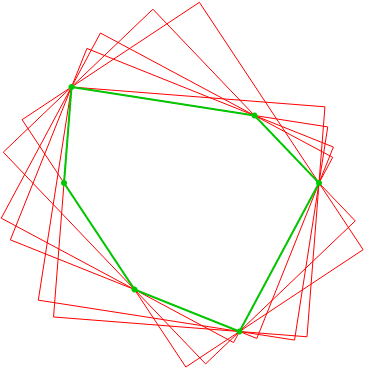
   1. Compute the area of the current rectangle.
   2. Update the minimum area and store the current rectangle if .
6. Repeat step 5 until all edges of the convex hull coincided once with one of the supporting lines.
7. Output the minimum area rectangle stored in step 5.2.

In practice, in every iteration the smallest angle between each caliper line and its associated, following convex hull edge is determined. Then, all caliper lines are rotated at once by and the associated convex hull edge of the caliper line enclosing the smallest angle is advanced to the next convex hull edge.

Wrap up

Rotating Calipers is a very elegant method for computing OMBBs in two dimensions. O’Rourke generalized it to three dimensions, yielding an algorithm of cubic runtime complexity. However, in practice approximation algorithms are used for three dimensional data because they’re usually faster. Beyond that, it's worth knowing the Rotating Calipers technique as it can be employed with minor changes to numerous other geometric problems. Depending on the programming language the implementation of the entire algorithm, including the convex hull computation, requires merely 150-200 lines of code. My sample implementation in Javascript can be found in my github repository.

---

1. H. Freeman, R. Shapira. Determining the minimum-area encasing rectangle for an arbitrary closed curve. Communications of the ACM, 18 Issue 7, July 1975, Pages 409-413 ↩

Making-of “Turtles all the way down”

Introduction

At Revision 2013 we (Brain Control) released our newest production Turtles all the way down, which won the 64k-intro competition. A 64k-intro is an audio-visual presentation computed in real-time, where all code and data has to be contained in a single executable which size may not exceed 64 KB. Five guys spent a year of most of their spare-time on creating this 65.536 bytes counting piece of binary data. In this making-of you can read about the process we went through creating this intro and about the used technology. The party version of the intro can be watched either as a video (embedded below) or by downloading the binary from here. Note that you need a fast graphics card for good experience. We tested it on NVIDIA Geforce GTX 570, 670, AMD Radeon HD7870 and some mobile graphics cards. On the compo machine (Geforce GTX 680) we experienced serious stuttering in the underwater scene. If you have similar problems please contact us.

Beginnings

A few weeks after Revision 2012 payne came up with the idea of making an intro zooming from microcosm all the way out to macrocosm. Inspiration came from the famous Powers of ten video (1977) and the opening scene of the movie Contact (1997). It did not take long to convince the other team members, namely hunta, pap, strepto and skyrunner, of this idea and to start working on the intro.

All content creation, animation, sequencing, and post-processing was done solely with our demo-tool Enigma Studio 4 (depicted in the figure below). You can download the tool, the project files and the full source code from our website. The current version counts around 100.000 lines of code, is written in C++ and uses Direct3D 11 and Qt 5. We have actively developed Enigma Studio since 2005. Thus, during the last year we could mainly concentrate on creating the intro content because most of user-interface and fundamental engine code had been written already. Though, we had to face a lot of new challenges such as memory management, size optimizing shaders, level-of-detail (LOD) techniques, L-systems for plants and animals, realistic skin generation for shells and finally the planet rendering. Besides the graphics, payne rewrote once more our software synthesizer Tunefish, but more on that later.

The next step was to distribute the work to be done. Skyrunner is the main musician of our team. Hence, he was in charge of doing the soundtrack. Pap undertook the job of bringing life to the underwater scene. This task meant rewriting the L-system code of Transplant so that even animals (nautilus and shells) could be generated. Additionally, a swarm behavior simulation and a skin texture generator had to be implemented. Strepto decided to work on the terrain and the planet rendering on the basis of ray-marching. Payne was responsible for the intro content and all special effects shaders. Last but not least, hunta cared about all the remaining engine and tool code, as well as porting the texture generator from the CPU to the GPU on the basis of compute shaders.

One year of work

Payne began working on the scenes taking place in microcosm: atoms, molecules, DNA and chromosomes. For that purpose hunta implemented a dynamic LOD system. It allowed showing a lot of geometry distributed over a wide depth range. Payne implemented a microscope shader, which gave all the beginning scenes a bluish look. After a while we realized that this look is too boring to be used for all beginning scenes. Therefore, payne created a different style for the first two scenes (atom and molecules). Below are some screenshots of the first attempts depicted.

This slideshow requires JavaScript.

The more payne progressed with the beginning scenes, the more the additional effects for the underwater and the planet scenes were needed. Pap progressed fast with his code. It was already early possible to generate undersea animals with very realistic skin textures and to simulate swarm behavior for the fish. The skin texture generation was based on the book Algorithmic beauty of sea shells. As pap knew his code and operators the best, he undertook the creation of the underwater scene geometry: placing plants, shells and nautilus, as well as simulating the fish swarms. All post-processing was added by payne. The caustics were faked by simply projecting an animated sum of two sine waves onto the ground and the water surface. The effect of sun shining diffusely through the water was faked by creating a halo post-processing shader, which added a shine over the final image. No real light source was used here. The same code was later used to create the sun glare in the space scenes. Below you can see some work-in-progress screenshots of the L-system and the underwater scene.

This slideshow requires JavaScript.

We knew early that every bit we could get would be needed to fit the whole code and data into 64 KB. Thus, it was clear that we also needed to come up with new ideas of how to synthesize audio.
Our old synthesizer Tunefish 3 was still relatively new and produced very satisfying sound. However, a range of different oscillators and the iFFT-based pad synth were simply too big. As throwing some of them out would have considerably reduced the final audio quality, payne sought a way to reduce the code size but not the audio quality. What if we found a way to produce all these nice sounds by coming up with just one type of oscillator instead of many? Classic oscillators can produce cool analog sounds, which we wanted to have. The iFFT-based pad synth algorithm can produce fat and rich sounds we did not want to miss neither. Though, it cannot produce the simple analog ones. Further more, it is not a real-time algorithm since it requires performing an iFFT on a table of 65536 frequencies. This was just not suitable for every kind of sound we needed, especially not for percussions. Consequently, the idea for the new generator of Tunefish 4 was born. What if we used an iFFT size that is

1. small enough to be evaluated in real-time,
2. still produces fat sounds and,
3. can also produce the simple square, sine and saw-tooth sounds that we all love?

After some days of experimenting it got clear that this was possible. The first attempts sounded more like alien sounds than anything we could possibly use to produce music. Though, it was only a question of time to get used to the new generator. What you hear in Turtles all the way down is not all Tunefish 4 is capable of by any means. There is still a lot of potential left in this approach. As the full source-code is public now, everybody can try out the VSTi and play with the knobs. Below is a screenshot of the Tunefish 4 VSTi depicted.

Let’s go back to the graphics. The terrain and the planet were both rendered via ray-marching, without using a single triangle. The difficulty with this approach was that we needed to change from a planar noise function for the terrain surface to a spherical one for the planet. Noise derivatives were used to slightly modify the traditional fractional Brownian motion (fBm) construction in order to generate a realistic surface. For performance reasons it was essential to ray-march as few steps as possible. This is why we used sphere tracing to step along the ray, starting only from the top of the atmosphere. Shadows, water reflections and water refractions were ray-marched using the same algorithm. The planet shader was combined with atmospheric scattering and clouds to increase the realism. Finally, some flock of birds and a space station rendered using traditional rasterization were combined with the planet by performing a per-pixel depth test. For that purpose the camera used in the terrain/planet shader had to match 1:1 the camera used for rasterization. Big thanks to IQ for his articles on noise derivatives, terrain marching and the Elevated making-of. Below are some work-in-progress screenshots depicted.

This slideshow requires JavaScript.

After the terrain and the planet scene the outer space begins. As we were not sure yet about the ending of the intro, payne started freely creating new artwork. There were plenty of ideas for the end of the intro:

• simply looping the intro,
• ending with a galaxy cluster, morphing into the shape of the Brain Control logo,
• the camera flies out of a computer screen.

In the end, mainly due to size problems, we opted for a simple fade-to-black after the credits. To cope with the large amount of geometry, especially for the asteroids, again hunta’s LOD system was used. Below there are screenshots of some space scenes depicted which didn’t make it into the final intro.

This slideshow requires JavaScript.

When payne began working on the space scenes we started having some bigger issues with the engine sub-systems. First of all, we exhausted more and more often the amount of available virtual memory and sometimes even video memory. The problem was that while working on the intro, all scenes and all intermediate operator results got loaded into memory over time. Therefore, hunta implemented an operator memory manager. The memory manager assigned every operator class which consumed a significant amount of memory (currently texture, mesh and scene-graph operators) a budget size. It automatically freed memory of those operators that were not part of any active operator stack, as long as their class’ budget size was exceeded. The operators to be freed were chosen in a least-recently-used (LRU) fashion.

The second problem was massive turn-around times between successive stack updates, when working on large (e.g. 4096×4096) textures. For such texture dimensions the CPU texture generator, especially the Perlin noise implementation, was too slow. Thus, hunta finally did what he wanted to do already for a long time. He ported all texture operators as compute shaders to the GPU. This boosted the performance dramatically and consequently the turn-around times shortened. As a result we obtained much nicer nebula textures.

Around two month before Revision 2013 nero/Still began to help us. He offered to do what he called “color consulting”. Though, it turned out to be much more than this. Besides creating plenty of overpaints giving us new ideas of how to tweak colors and light to increase the overall scene quality, he provided tons of valuable feedback and tips on how to improve the flow and the style of the intro. Below you can see some of the original scenes and the corrections as overpaints as proposed by nero.

This slideshow requires JavaScript.

At the party place

Usually, we do a one week coding meeting directly before a demo party if we plan to release something at it. These meetings are of great value as they allow us to fully concentrate on the production. This year we did it again and progressed so well that we believed we would have plenty of time for boozing at Revision. It turned out we were wrong. After arriving at the party place we directly tested our intro on the compo machine. Unfortunately, it turned out that there was still a hell lot of work to do, if we wanted to make it for the deadline. We faced horrible stuttering issues in the underwater scene, discontinuities in the terrain scene and geometry popping issues in the chromosomes, DNA and molecules scenes. After three days of non-stop coding, we luckily managed to fix most of the issues. Unfortunately, we were not able to fix the stuttering, because this problem only appeared on the compo machine. After some blind attempts to fix it we simply ran out of time.

While hunta worked on fixing the issues mentioned above, pap and payne continued crunching even more content into the 64 KB. Pap worked hard on further size-optimizing the intro. This time he focused on the shaders. The first thing we did after Revision 2012 was changing from binary shaders to text shaders; size optimized by Shader Minifier. This approach saved us around 4 KB of compressed size in the player executable, but pap believed that there could be done more. Therefore, he crafted our own custom shader cruncher that applied a couple of more optimizations than Shader Minifier. It replaced e.g. all HLSL keywords by short macros and added a #define for that replacement to the shader, or it minified the variables declared in constant buffers. Our own shader cruncher saved another 2-3 KB just two days before the deadline right at the party place. This allowed us to add the space station and the space ships. Overall, 58 shaders were used in the intro with a total, uncompressed size of 170 KB (comments counted). Below there are some work-in-progress screenshots of the space station depicted.

This slideshow requires JavaScript.

All in all we are very happy about the first place at Revision 2013. Though, for us it was even more important that Brain Control as a demo group did the next step when it comes to teamwork, technology, design and direction. We are already looking forward to the next 64k-intro competition and hope to see you at the next demoparty!

Hidden HLSL performance hit: accessing unpadded arrays in constant buffers

Introduction

From shader model 4 on in Direct3D 10/11 shader constants are grouped into constant buffers (cbuffers) to reduce API overhead and bandwidth required to pass shader constants from CPU to GPU. When declaring cbuffer elements certain packing rules are applied. First of all, cbuffer elements are aligned to 4-byte boundaries. Additionally, the shader compiler attempts to pack multiple cbuffer elements into float4 variables to save size. When an element straddles the current float4, it is put into the next float4. Look at the following example:

cbuffer // size is 28 bytes (1x float4 + 1x float3)
{
    float2 a;   // start of first float4, offset=0, size=8
    float  b;   // part of first float4, offset=8, size=4
//  float  pad; // invisible padding, offset=12, size=4
    float3 c;   // start of second float4, offset=16, size=12
                // (float3 does not fit into rest of last float4)
};

One exception to this rule are arrays declared inside cbuffers. For each element of such arrays a full float4 is allocated, independent of the real array type. This saves ALU instructions for the address offset computations. However, it can lead to problems when reading from those arrays as they are not tightly packed anymore, but the data copied from CPU mostly is. Furthermore, as there is a maximum number of available cbuffer elements (currently 4096 float4 variables) it can be necessary sometimes to avoid wasting any cbuffer space. Look at the following example.

cbuffer
{
    float vals[32]; // consumes 500 bytes, not 128 bytes
};

The size of the cbuffer above is 500 bytes, not 128 bytes as one might assume. Between every two array elements there are three padding float variables inserted. Note, that after the last array element no padding is done anymore. This is why the size is 500 bytes, not 512 bytes ((31×4+1)×4 bytes = 500 bytes).

Array access difficulties

Now, if a tight block (unpadded) of 32 float values (128 bytes) is copied to the cbuffer, only the very first float at index 0 will be correctly read in the shader, because the cbuffer padding offsets every other array access after the first one. To avoid this the cbuffer from the previous example could be declared like this:

cbuffer
{
    float4 vals[8]; // 8*4=32 floats = 128 bytes
};

Using that declaration the vals array is tightly packed, because no padding is performed. Thus, it contains exactly the data which is copied over from the CPU. However, now it is not possible anymore to address the individual float array elements without performing additional indexing calculations.

float flt = vals[i>>2][i&3];

To get rid of the indexing calculations the vals array could be "casted" (Is it really a cast? We come back to that in the next section.) into a float array. That way it is possible to read the tightly packed float data from vals without explicitly performing any additional indexing.

float fltArr[32] = (float[32])vals;
float flt = fltArr[i];

Hidden inefficiencies?

Even though, it is convenient to access a block of tightly packed memory in a shader using the syntax above, there is an associated overhead when doing so. Arbitrarily accessing individual float4 elements by an index variable, e.g. a loop counter, is a lot less efficient, because of additional indexing overhead. Let's consider the following shader compiled with -O3. It consists of four loops, each adding count elements of a float array from a cbuffer. The first loop obtains the float elements from a padded array, the other three loops from a tightly packed one.

cbuffer
{
    float  vals[512];  // for loop 1
    float4 tight[128]; // for loop 2 and 3
    uint   count;      // <= 512
};

float4 main(float4 hpos: SV_Position): SV_Target0
{
    float sum = 0.0f;
    uint i;

    for (i=0; i<count; i++) // loop 1
        sum += vals[i];

    for (i=0; i<count; i++) // loop 2
        sum += tight[i>>2][i&3];

    float valsLin[512] = (float[512])tight;
    for (i=0; i<count; i++) // loop 3
        sum += valsLin[i];

    for (i=0; i<count>>2; i++) // loop 4
        sum += tight[i].x+tight[i].y+tight[i].z+tight[i].w;

    return float4(sum, sum, sum, 1.0f);
}

The above shader was compiled four times. Each time everything which is not required to compile the respective loop was commented out. The generated code for each loop differs significantly concerning performance. Let's look at the generated assembly code for each loop, starting with the first one.

// loop 1
mov r0.xy, l(0,0,0,0)
loop
  uge r0.z, r0.x, cb0[511].y      // r0.z = r0.x >= count?
  breakc_nz r0.z                  // yes => break
  add r0.y, r0.y, cb0[r0.x + 0].x // r0.y += cb0[r0.x].x
  iadd r0.x, r0.x, l(1)           // r0.x++
endloop

This is the fastest way to iterate over all array elements. All instructions inside the loop except the add instruction are loop overhead. Though, the array elements are padded and thus, copying to the cbuffer from the CPU has to account for this. The disassembly of the second loop is shown below.

// loop 2
dcl_immediateConstantBuffer { { 1.000000, 0, 0, 0},
                              { 0, 1.000000, 0, 0},
                              { 0, 0, 1.000000, 0},
                              { 0, 0, 0, 1.000000} }
mov r0.xy, l(0,0,0,0)
loop
  uge r0.z, r0.x, cb0[128].x // r0.z = r0.x >= count?
  breakc_nz r0.z             // yes =>; break
  and r0.z, r0.x, l(3)       // r0.z = r0.x&3 (mod 4)
  ushr r0.w, r0.x, l(2)      // r0.w = r0.x>>2 (div 4)
  dp4 r0.z, cb0[r0.w + 0].xyzw, icb[r0.z + 0].xyzw // select
  add r0.y, r0.z, r0.y       // r0.y += r0.z
  iadd r0.x, r0.x, l(1)      // r0.x++
endloop

Here, the shader compiler generated code to dynamically select the r0.z^th component of the r0.w^th float4. The selection is performed based on a dot-product between the current float4 and a float4 from an immediate constant buffer, effectively zeroing all unwanted components. With this approach it is possible to access a non-padded array, though it requires three additional instructions inside the loop. Next, we have a look at the third loop.

// loop 3
dcl_indexableTemp x0[512], 4
mov x0[0].x, cb0[0].x // copy each array element into its
mov x0[1].x, cb0[0].y // own float4 register. all elements
mov x0[2].x, cb0[0].z // are copied, independent of the value
mov x0[3].x, cb0[0].w // of count
...
mov x0[508].x, cb0[127].x
mov x0[509].x, cb0[127].y
mov x0[510].x, cb0[127].z
mov x0[511].x, cb0[127].w
mov r0.xy, l(0,0,0,0)
loop
  uge r0.z, r0.x, cb0[128].x // same as loop 1
  breakc_nz r0.z
  mov r0.z, x0[r0.x + 0].x
  add r0.y, r0.z, r0.y
  iadd r0.x, r0.x, l(1)
endloop

It turns out that the syntactically easiest way to access the tightly packed float array is the least efficient. What might be interpreted as some sort of type-cast turns out to be a very costly copy operation. Every single float from the vals array gets copied into a padded temporary array x0. The loop it-self is identical to the first loop, accessing the temporary array x0. It follows the analysis of the fourth loop.

// loop 4
ushr r0.x, cb0[128].x, l(2) // divide count by 4
mov r0.yz, l(0,0,0,0)
loop
  uge r0.w, r0.y, r0.x                  // r0.w = r0.y >= count?
  breakc_nz r0.w                        // yes => break
  add r0.w, cb0[r0.y+0].y, cb0[r0.y+0].x // r0.w = sum of 4
  add r0.w, r0.w, cb0[r0.y + 0].z       // float4 components
  add r0.w, r0.w, cb0[r0.y + 0].w
  add r0.z, r0.w, r0.z                  // r0.z += r0.w
  iadd r0.y, r0.y, l(1)                 // r0.y++
endloop

This is the fastest way to calculate the sum of an unpadded float array. By explicitly specifying the components to sum up, one gets rid of the dp4 instruction and the additional immediate cbuffer for masking. However, the indexing is of course not arbitrary anymore. The components are explicitly stated and thus, the compiler can generate optimal code. There are cases when that approach surely won't work.

Summary

Accessing unpadded, multi-component variables by an index variable can result in very poorly performing code. Usually, the best way is to go for padded arrays. Though, sometimes it can be necessary to tightly pack arrays in cbuffers. Either if the amount of data to be passed is large, or the way the memory block is copied to the cbuffer cannot be changed to account for the padding. In that case the access pattern as seen in the second loop should be favoured.